Benchmarks#

Several harnesses ship with the repo, covering raw throughput, recall, E-value significance, and the epitope-detection formalism. Most bootstrap realistic TCR CDR3 sequences from OLGA (if installed) and otherwise fall back to seeded random sequences. Figures are rendered to SVG with gnuplot.

Reproducible tables and the CI oracle#

Benchmarks are split into two stages so results are reproducible and regression-checked:

Table producers (bench/tables/*.py, driven by bench/tables/make_tables.sh) run the compiled seqtree from the current repo on a fully seeded synthetic workload — no network, no OLGA — and write TSV tables. Because every number is integer-derived, the output is identical on every platform and doubles as a committed oracle.
Plot scripts (bench/plots/*.py, driven by bench/plots/make_plots.sh) read those TSVs and render SVGs. They never run seqtree, so plotting never re-measures anything.

bash bench/tables/make_tables.sh --perf   # regenerate tables + perf baseline
bash bench/plots/make_plots.sh            # render figures from the tables

CI regenerates the table on the freshly built extension and fails if it differs from the committed oracle (tests/python/test_oracle_tables.py); a deliberate change means rerunning the driver and committing the new table. A separate perf check (test_perf_regression.py, RUN_PERF=1) asserts build/search time and peak RSS stay within a threshold of perf_baseline.tsv — loose on time (runners vary) and tight on memory (machine-independent).

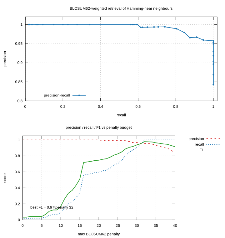
The retrieval table scores BLOSUM62-weighted seqtrie search against brute-force Hamming-near ground truth and sweeps the penalty budget into a precision/recall/F1 curve:

precision-recall and precision/recall/F1 vs penalty budget for BLOSUM62 retrieval

C++ (raw throughput + scaling)#

cmake -S . -B build -DSEQTREE_BENCH=ON && cmake --build build
./build/seqtree_bench 1000 10000 100000 1000000

Reports build time, peak RSS, single-query latency (median / p99), batch throughput, and thread scaling, followed by a two-engine comparison and per-call alignment cost.

Python (methods + recall)#

bench/bench_methods.py compares seqtm vs seqtrie across reference sizes, edit scopes, and budgets (edit count and BLOSUM62 score), plus alignment-fetch cost:

python bench/bench_methods.py
env RUN_BENCHMARK=1 python bench/bench_methods.py --sizes 100000 1000000

bench/bench.py measures recall against ground truth on the AIRR VDJdb table (queries are mutated references with known parents), with throughput and peak RSS:

python bench/bench.py
env RUN_BENCHMARK=1 python bench/bench.py --sizes 1000000 --queries 1000000 --threads 16

E-value benchmark#

bench/bench_evalue.py is the true E-value benchmark. For a target repertoire (VDJdb, antigen-selected) scored against the airr_control background, at each scope/budget it reports the number of neighbours (distinct hits, excluding exact/self matches — the queries are members of the target, so the self-match is dropped per the punctured-null lemma), the exact self-hits removed, the number of collisions (references re-reached via a different edit path — non-zero only for seqtm with indels), and the fraction of neighbours called significant both at fixed E-value cutoffs and after a Benjamini–Hochberg FDR correction across the query family:

python bench/bench_evalue.py
env RUN_BENCHMARK=1 python bench/bench_evalue.py --target-size 200000 --control-size 2000000

The discriminating result is the contrast between query sets: antigen-selected VDJdb queries produce orders of magnitude more neighbours and are largely significant (BH FDR < 0.05), whereas background (control) queries produce almost none and survive no correction. The smallest resolvable E-value is $N/M$, so finer fixed cutoffs (E < 0.01) require a control much larger than the target (the RUN_BENCHMARK tier uses $M = 2{,}000{,}000$); the BH correction is what makes the fixed-cutoff fractions trustworthy at small control sizes.

Comprehensive matrix#

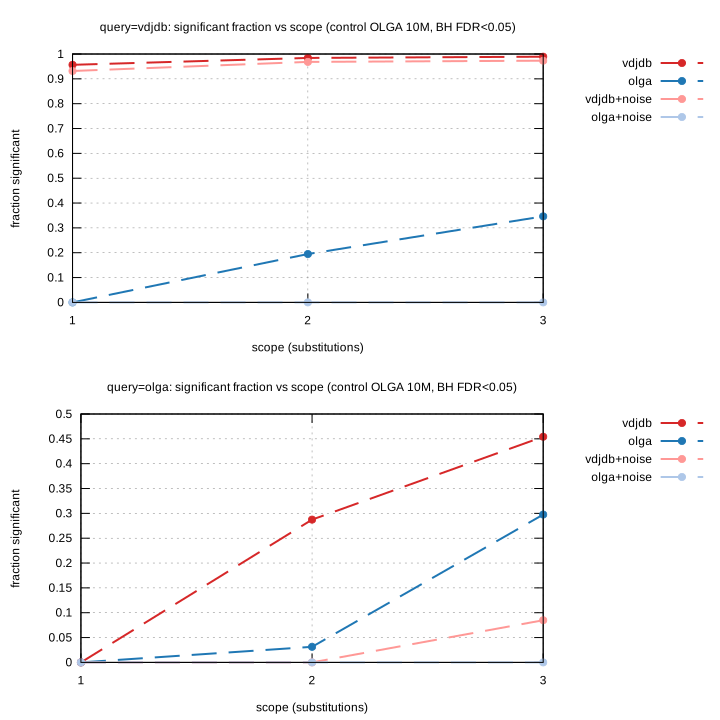
bench/bench_evalue_matrix.py sweeps the full grid — reference set (vdjdb / olga / vdjdb+noise / olga+noise, all built to the same size $N$), background control (OLGA 1M / 2M / 10M), query set (vdjdb / olga), and scope (1–3 substitutions) — and emits a TSV table plus evalue_matrix.svg:

python bench/bench_evalue_matrix.py                       # control 1M
env RUN_BENCHMARK=1 python bench/bench_evalue_matrix.py   # controls 1M / 2M / 10M

The signal is structural: vdjdb queries against a vdjdb reference are ~0.87–0.98 significant (BH), vdjdb+noise stays ~0.77–0.97 (real clusters survive 50 % dilution), while olga, olga+noise, and all cross combinations sit at ~0. The naive E < 1 column over-calls (e.g. olga-vs-olga reads 1.0) where BH reads 0.0 — a direct demonstration that the multiple-testing correction is what separates genuine convergence from background.

$significant fraction across reference/control/query/scope combinations$

Epitope detection complexity#

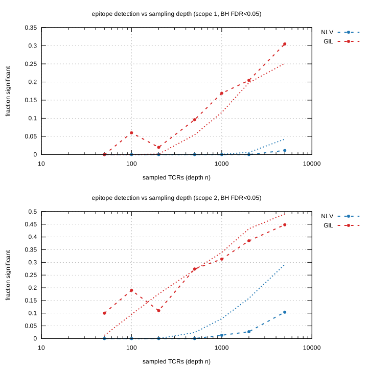
bench/bench_epitope.py tests the detectability formalism on two HLA-A*02 epitopes of opposite repertoire structure: GIL (GILGFVFTL, one dominant convergent cluster) and NLV (NLVPMVATV, many diverse small clusters). It reports each epitope’s within-set neighbour density, degree, and cluster sizes, then subsamples to depth $n$ and plots the fraction called significant (BH FDR < 0.05) against the degree-distribution prediction of Eq. (φ) in the appendix:

python bench/bench_epitope.py --scopes 1 2

At scope 1, GIL (ρ = 3.4×10⁻⁴, largest cluster 896 = 17 % of the set) is ~20–30 % recovered by $n\sim10^3$ sampled TCRs, while NLV (ρ = 2.8×10⁻⁵, largest cluster 152 = 1.2 %) stays below 5 % even at $n\sim5\times10^3$ — detection complexities differing by an order of magnitude purely from repertoire structure. See appendix/evalue.tex §”Epitope detection complexity”.

$significant fraction vs sampled depth for GIL and NLV epitopes$

MHC-allele guessing#

bench/bench_mhc_guess.py evaluates the reverse problem — peptide → presenting allele — as a per-(peptide, allele) binary task (exactly how vdjmatch scores TCR-antigen specificity), for class I and class II, human and mouse separately. Each held-out peptide’s presentation (anchor) signature is widened until it has 10–100 non-exact neighbours; the neighbours’ alleles are voted. Two scores come off the tally: the vote fraction k_a/n ranks alleles (a posterior, robust to panel skew), and the per-allele E-value (binomial enrichment vs background) gives a confidence that rejects random noise. Class II uses the register trick — commit to the single best 9-mer core register (layout.presentation_features(register="anchored")) so an allele’s peptides share a consistent P1/P4/P6/P9 signature:

python bench/bench_mhc_guess.py --pmhc /path/to/pmhc_full.tsv.gz

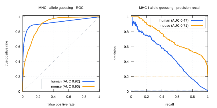
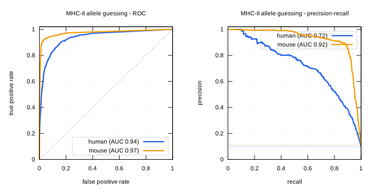
On pmhc_data the vote-fraction ranking gives ROC-AUC ≈ 0.90–0.98 with PR-AUC far above the prevalence baseline, for both classes and both species (MHC-I human 0.92 / mouse 0.90; MHC-II human 0.94 / mouse 0.98), and top-1 accuracy 0.58–0.89. The confidence E-value separates real peptides from length-matched random peptides. This works only with anchor features — TCR-facing homology carries no allele information (AUROC ≈0.5), confirming MHC restriction lives in the anchors.

MHC-I allele-guessing ROC and precision-recall, human vs mouse

MHC-II allele-guessing ROC and precision-recall, human vs mouse

TCR-beta benchmark (gnuplot figures)#

bench/bench_gnuplot.py is the main benchmark. It measures two reference families separately, so the effect of sequence structure is visible rather than averaged away:

olga — OLGA-generated human TRB CDR3 (a generative model, no antigen motif); queried with 1000 fresh OLGA TRB sequences.
vdjdb — VDJdb CDR3 mutated (real antigen-specific receptors, with shared motif structure); queried with 1000 held-out VDJdb CDR3.

Both families are expanded by substitution-mutation to each target size. Timings are over the 1000 queries. Figures are vertically stacked two-panel SVGs; seqtm is drawn with a long dash and seqtrie with a dash-dot, and the reference family is encoded by colour.

python bench/bench_gnuplot.py                       # fast tier: 10k / 100k
env RUN_BENCHMARK=1 python bench/bench_gnuplot.py   # full tier: 10k / 100k / 1M / 10M

Each figure is written to bench/figures/<key>.svg (+ per-panel .tsv). Requires gnuplot and olga-generate_sequences on PATH (pip install olga). The scaling, matrix and per-op figures span all reference sizes; the edit-budget sweeps (scope, selectivity, collisions) run at one representative size to stay tractable.

A note on engine semantics: at an edit budget e, seqtm explores the Hamming ball (max_subs=e, substitutions only — the dominant TCR diversity/error mode) while seqtrie explores the edit-distance ball (max_total_edits=e, substitutions and indels). They answer subtly different questions, which shows as a higher match count for seqtrie at the same e.

Scaling and parallelism#

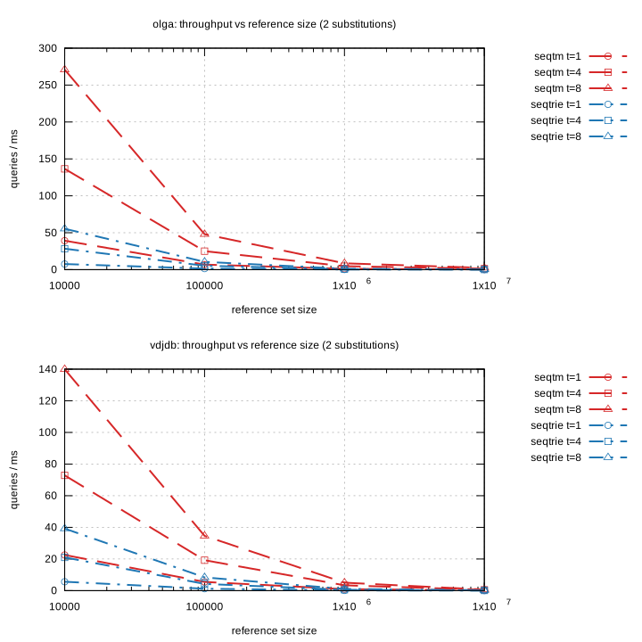
Throughput (queries per millisecond) versus reference-set size, for both engines at 1, 4, and 8 threads (fixed scope: 2 substitutions), with the olga family on top and vdjdb below. Batches parallelize near-linearly to 8 cores (~6.5–7×):

throughput vs reference size per engine and thread count, olga and vdjdb

Edit budget#

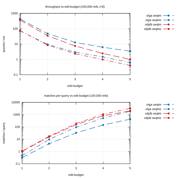
Cost (top) and selectivity (bottom) as the edit budget grows from 1 to 5. Throughput is governed by scope far more than by reference-set size, and the match count grows steeply — by e = 5 a query already pulls hundreds (seqtm Hamming ball) to thousands (seqtrie edit ball) of neighbours, so loose budgets are rarely useful:

Matrix scoring (BLOSUM62 / PAM250 / custom)#

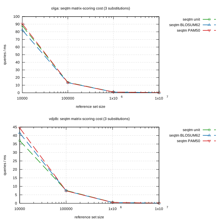
seqtm scores substitutions through a substitution matrix, reporting the best (minimum-penalty) score across all alignments to each reference. The time overhead of matrix scoring is small (within ~5–10 % of unit cost — one table lookup replaces a character compare), for both families:

seqtm throughput unit vs BLOSUM62 vs PAM250, olga and vdjdb

The built-in matrices are identity, BLOSUM62, PAM250, PAM100 and structural (a Miyazawa–Jernigan interaction-strength similarity — residues are close when their MJ contact strengths q(a)=mean_b e(a,b) match, separating strong hydrophobic F W C L Y M I V from weak polar/charged S Q D E K interactors; Košmrlj et al., PNAS 2008, doi:10.1073/pnas.0808081105); a custom matrix is supplied via SubstitutionMatrix.from_similarity (row/column order from seqtree.amino_acids()).

Selectivity and collisions#

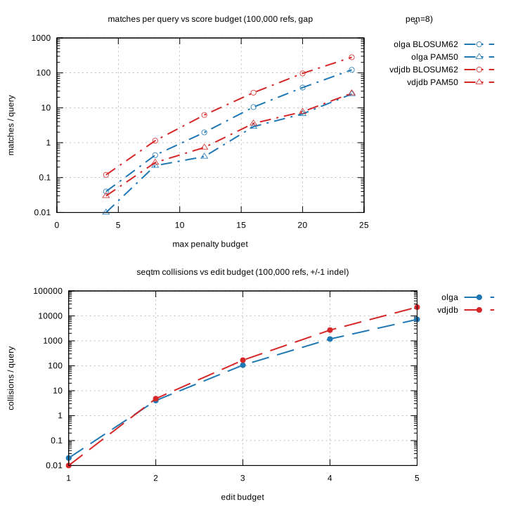
Top: matches per query versus the seqtrie max_penalty budget — PAM250 is stricter than BLOSUM62 at equal budget. Bottom: collisions — how often seqtm’s branch-and-bound re-reaches the same reference via a different edit path (reported by Index.collisions_batch). Substitution-only search never collides; once indels are allowed, collisions rise with the edit budget, and the motif-rich vdjdb family collides far more than olga because shared structure makes a reference reachable by many distinct edit paths:

matches per query vs penalty budget, and seqtm collisions per query vs edit budget

Per-operation costs#

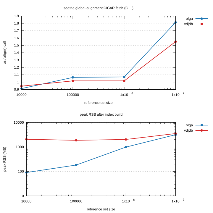
Top: fetching a global-alignment CIGAR (the C++ Needleman–Wunsch in Index.align) is on-demand and about a microsecond per call, roughly flat in reference count. Bottom: peak resident memory after the index build, which scales with the reference count (the trie is shared by both engines):

Indicative numbers#

Apple M3, OLGA TRB references, 1000 queries, 8 threads (bench/bench_gnuplot.py, full tier):

metric	10k	100k	1M	10M
seqtm, 2 subs (q/ms)	~271	~48	~8.6	~2.4
seqtrie, edits≤2 (q/ms)	~55	~11	~1.2	~0.28
align CIGAR fetch (µs)	~0.9	~1.1	~1.1	~1.8
peak RSS (MB)	~91	~183	~990	~3170

The 8-thread speed-up is ~6.5–7×; matrix scoring stays within ~5–10 % of unit cost across all sizes.

Takeaway#

Throughput is governed by scope (edit budget) far more than reference-set size, parallelizes near-linearly to 8 cores, and matrix scoring is nearly free. Sequence structure matters: the motif-rich vdjdb family is denser and collides more under indels — enumeration cost ultimately depends on reference redundancy (see Roadmap).