Mathematical foundations#

This page is one argument, read top to bottom. It starts from the reason a set of immune receptors has no natural vector representation, builds the one it does have in three steps, shows what that object knows and what it cannot know, then repairs the one premise that fails on real data. Each section ends with the calls that compute what was just derived, so the page doubles as a map of the library — but the order is the order of the derivation, not the order of the modules.

Where a step is stated as a proposition, the label in parentheses (prop:kme, eq:rff, …) is the label it carries in the theory appendix of the companion manuscript, so a docstring, this page and the appendix all name the same result. Numbers quoted as measured are empirical results from the benchmark programme, reproduced here because they decide a design question.

The argument in one page #

A repertoire is an unordered set of variable size, so no fixed-dimensional map is even defined on it. Everything downstream follows from fixing that. → The problem, and the shape of the solution
A sequence becomes a point by its distances to a fixed panel of reference receptors. The map is Lipschitz, so Euclidean geometry in that space tracks alignment distance. → Step 1 — a sequence becomes a point
A sample becomes a measure on those points. This single quotient removes order and length at once, and it is the only way an embedding can be order-invariant. → Step 2 — a sample becomes a measure
Normalising the measure to total mass 1 buys mixture linearity: a point between two sample embeddings is the embedding of a real pooled repertoire. Everything in The algebra that survives and every generative operation rests on this one property. → Why normalise: the mixture property
A measure becomes a vector through a characteristic kernel. The kernel mean is an empirical characteristic function, its distance is the MMD, and it converges at the Monte-Carlo rate in effective sample size. → Step 3 — a measure becomes a vector
That vector already contains the classical statistics: richness and Shannon are recoverable from it, and Rao’s quadratic entropy is exactly 1 − ‖Φ₁‖². The right question is therefore recoverability, not competition. → What the vector already knows
But claim 3 assumed the weights are frequencies. At RNA-seq depth they are not — they are 1/n for a technical draw size. Repairing that gives a sub-probability measure, a principled location for what was never observed, and a signed contrast. → When the sample is not a probability distribution
The failure is variance, not bias, and its scale is estimable: κ = σ²/τ² is the sample size at which sampling noise equals biological signal. → How much of a sample can be trusted
Mixture linearity then licenses two further operations exactly — compartment decomposition and rarefaction — the second with a closed-form identity for its own noise. → The algebra that survives
The same points support a clone-level test (local density against a background), and the same vectors support cohort-level read-outs and generation. → Back to the single clone: local density, From vectors to answers, From vectors back to biology
Every transformation applied to Φ keeps some of these properties and breaks others. The final table is the contract. → The contract: which transformation preserves what

Notation #

symbol	meaning
\(\sigma\)	a clonotype: the triple (`junction_aa`, `v_call`, `j_call`)
\(a_\sigma\)	its clone size (`duplicate_count`); \(N = \sum_\sigma a_\sigma\) the read total
\(S\)	a repertoire — the multiset \(\{(\sigma, a_\sigma)\}\); \(n = \|S\|\) its richness
\(\varphi(\sigma) = z_\sigma \in \mathbb{R}^p\)	the clonotype embedding (`TCREmp`)
\(g\)	the clone-size transform; \(w_\sigma = g(a_\sigma)/\sum_\tau g(a_\tau)\)
\(\rho_S\)	the sample measure \(\sum_\sigma w_\sigma \delta_{z_\sigma}\)
\(k, \psi\)	the kernel and its random-Fourier feature map, \(k(z,z') \approx \psi(z)^\top\psi(z')\)
\(\Phi_1(S)\)	the kernel mean embedding \(\sum_\sigma w_\sigma \psi(z_\sigma)\)
\(f_1, f_2, f_{3+}\)	the number of clonotypes seen exactly once, twice, three or more times
\(M_0\)	the missing mass — total frequency of the clonotypes never drawn
\({}^qD\)	the Hill number of order \(q\); \(n_{\text{eff}} = (\sum_\sigma w_\sigma^2)^{-1}\)

The problem, and the shape of the solution #

A repertoire is a set of receptors with clone sizes: unordered, and of a size that varies by orders of magnitude between samples. Raw inputs therefore live in

\[\bigsqcup_{n \ge 1} (\mathbb{R}^p)^n / \mathfrak{S}_n ,\]

the disjoint union over all lengths of tuples-up-to-reordering. No fixed-dimensional map is even defined there, so there is nothing to feed a model — and the two obstructions are different in kind: order is a symmetry, length is a dimension mismatch. Any fix has to dispose of both.

The construction below disposes of them in three steps, and the point of splitting it into three is that each step preserves a named property, and each property is what licenses one class of later operation:

Read the dotted notes as the reason each step exists. Step 1 makes distance meaningful, step 2 makes the object well-defined and interpolable, step 3 makes comparison a statistical distance. Lose any one property and a whole class of operation goes with it — which is why the last section of this page is a table of exactly what each downstream transformation keeps.

Step 1 — a sequence becomes a point #

Before a set can be summarised, its elements need coordinates in which nearness means biological similarity.

The prototype embedding #

Fix a panel of \(K\) reference clonotypes \(\{\pi_1,\dots,\pi_K\}\). A query clonotype is represented by its distances to the panel, in three separate geometries concatenated (eq:embedding):

\[\varphi(\sigma) \;=\; \big(\, d_{\mathrm{junc}}(\sigma, \pi_k),\; d_{V}(\sigma, \pi_k),\; d_{J}(\sigma, \pi_k) \,\big)_{k=1}^{K} \;\in\; \mathbb{R}^{3K}.\]

The junction term is the gap-block alignment score of seqtree (BLOSUM62 Gram penalty, gap placements \((3,4,-4,-3)\)); the V and J terms are baked germline region distances (CDR1/CDR2 included), looked up per allele with a cascade fallback. Note for later that every coordinate is a distance, so \(\varphi\) is all-positive — a fact with a practical consequence in The contract: which transformation preserves what.

Why this is a coordinate system and not a trick #

For a metric \(d\), the map \(\sigma \mapsto (d(\sigma,\pi_k))_k\) is 1-Lipschitz in each coordinate (prop:lipschitz), giving a two-sided grip on the original distance:

\[\frac{1}{\sqrt{K}}\,\|\varphi(\sigma) - \varphi(\tau)\|_2 \;\le\; d(\sigma,\tau) \quad\text{and}\quad d(\sigma,\tau) \;\ge\; \max_k \big| d(\sigma,\pi_k) - d(\tau,\pi_k) \big| .\]

So Euclidean distance in embedding space is a lower bound on — and empirically a close proxy for — the alignment distance it replaces. The consequence that matters in practice: the panel does not have to be biologically special, it only has to span. Measured, the pairwise geometry induced by two independent prototype draws agrees at \(R = 0.922\) at \(K = 100\), \(0.990\) at \(K = 500\) and \(0.997\) at \(K = 2000\); real and model-generated panels agree at \(R = 0.965\). From \(K \approx 500\) up, which prototypes were drawn is not what a result rests on.

Two prototype panels are nevertheless two different coordinate systems, and distances across them are not comparable. That is why every serialisable object in the library carries a prototype hash and refuses to load against a different panel.

Squared versus root metric #

metric="squared" (the default, and the published space) uses \(d\); metric="sqrt" uses \(\rho = \sqrt{d}\). The latter is the metrically tidier choice — \(\sqrt{d}\) satisfies the triangle inequality for a wider class of \(d\) and makes the space of negative type, hence Hilbert-embeddable (prop:schoenberg) — and benchmarked as a wash, so the default stays put.

Call. mir.embedding.tcremp.TCREmp.embed() → (n, 3K); mir.distances.junction.junction_distance_matrix() for the junction block alone.

Step 2 — a sample becomes a measure #

We have a point per receptor. A sample is a set of them, and a set of variable size still has no vector. One quotient fixes both obstructions at once.

The quotient that removes order and length #

Pass from the tuple to the empirical measure (def:sampmeasure, eq:sampmeasure):

\[\rho_S \;=\; \sum_{\sigma \in S} w_\sigma\, \delta_{z_\sigma}, \qquad w_\sigma = \frac{g(a_\sigma)}{\sum_\tau g(a_\tau)} .\]

\(\rho_S\) is a single point of \(\mathcal{P}(\mathbb{R}^p)\) whatever \(n\) is — the dimension mismatch is gone because the object no longer has a dimension that depends on \(n\) — and it is manifestly unchanged by reordering. The converse is the design constraint: a sample embedding is order-invariant iff it factors through \(\rho_S\) (prop:sampinv). Anything that does not factor through the measure is reading the input order.

Cardinality is not lost in the quotient, only relocated: it re-enters explicitly as richness \({}^0D = n\) inside the diversity block. The embedding sees how many clonotypes there are without letting that count set its dimension.

The clone-size transform #

Clone sizes are Zipf-heavy, so the choice of \(g\) decides whether one hyperexpanded clone owns the vector. A concave \(g\) tames the tail:

`weight=`	\(g(a)\)	character
`"log2p1"` (default)	\(\log_2(1+a)\)	concave; a clone at \(10^6\) reads outweighs a singleton \({\sim}20\times\), not \(10^6\times\)
`"log1p"`	\(\ln(1+a)\)	same shape, natural base
`"anscombe"`	\(\sqrt{a + 3/8}\)	variance-stabilising for Poisson counts
`"duplicate_count"`	\(a\)	linear; the frequency measure, tail-dominated
`"distinct"`	\(1\)	presence only; then \(n_{\text{eff}} = {}^0D\)

Why normalise: the mixture property #

Dividing by \(\sum_\tau g(a_\tau)\) looks like a cosmetic choice and is not. Because the construction is linear in the clone-weight measure, a partition of a repertoire into sub-populations \(c\) with weight shares \(\pi_c\) satisfies

(1)#\[\rho_S = \sum_c \pi_c\, \rho_c \quad\Longrightarrow\quad \Phi(S) = \sum_c \pi_c\, \Phi(c), \qquad \pi_c = \frac{\sum_{\sigma \in c} g(a_\sigma)}{\sum_\tau g(a_\tau)} ,\]

an identity, not an approximation. Two corollaries used repeatedly below. Pooling two samples gives \(\Phi(S \cup T) = (N_S\Phi_S + N_T\Phi_T)/(N_S+N_T)\) — exactly linear interpolation, so a point between two sample embeddings is the embedding of a real pooled repertoire. And any partition can be decomposed after the fact, which is what makes Compartments and the dilution factor and Rarefaction, and the exact Rao gap exact rather than approximate.

The unnormalised sum has no such property: its midpoint is the embedding of nothing. Nor does one lose anything by normalising, since normalise-or-not is exactly one scalar (\(\Phi_{\text{sum}} = N\,\Phi_{\text{mean}}\)) — so keeping the mean and carrying \(\log N\) as its own channel strictly dominates the plain sum, and measured, it does.

Call. mir.repertoire.RepertoireSpace.sample_cloud() → \((Z, w)\).

Step 3 — a measure becomes a vector #

A measure is well-defined but infinite-dimensional. To compare two of them with a number, embed them in a Hilbert space where the inner product is a kernel.

An empirical characteristic function #

Take a shift-invariant kernel. By Bochner’s theorem it is the Fourier transform of a finite measure \(\Lambda\),

\[k(z,z') \;=\; \int e^{i\omega^\top (z-z')}\, d\Lambda(\omega),\]

so sampling frequencies \(\omega_j \sim \Lambda\) approximates the kernel by an explicit feature map (eq:rff):

\[\psi(z) \;=\; \sqrt{\tfrac{2}{D}}\, \big(\cos(\omega_j^\top z + b_j)\big)_{j=1}^{D}, \qquad \omega_j \sim \mathcal{N}(0, \ell^{-2} I),\;\; b_j \sim \mathcal{U}[0,2\pi],\]

with \(\mathbb{E}[\psi(z)^\top\psi(z')] = k(z,z')\) (Rahimi–Recht). The \(\cos(\omega^\top z + b)\) form is real-inner-product bookkeeping; what is actually being computed is transparent (eq:ecf):

\[\sum_\sigma w_\sigma e^{i\omega_j^\top z_\sigma} \;=\; \int e^{i\omega_j^\top z}\, d\rho_S(z) \;=\; \widehat{\rho_S}(\omega_j),\]

the sample’s empirical characteristic function, evaluated at \(D\) random frequencies. So \(\Phi_1(S) = \sum_\sigma w_\sigma \psi(z_\sigma)\) is a finite sketch of a complete description of \(\rho_S\).

That the summary is codebook-free follows from the same line: no clustering, no vocabulary, no \(K\) to tune (prop:codebook). The bandwidth \(\ell\) is calibrated to the one-substitution embedding scale \(r_1\) (mir.density.calibrate_radius()), so the kernel resolves about one CDR3 mutation — and the same \(r_1\) reappears as the radius in Back to the single clone: local density.

Why the characteristic function and not a moment-generating one #

This is the step where the heavy tail could have destroyed everything. An \(e^{t^\top z}\) feature would be dominated by the single largest clone and need not even converge on a Zipf distribution, whereas \(|e^{i\omega^\top z}| = 1\) is bounded, always exists, and is robust to a hyperexpanded clone. And by Lévy uniqueness the characteristic function is a complete invariant: two measures with the same one are the same measure. That is exactly the requirement that the kernel be characteristic, and it is what makes the next paragraph a metric statement rather than a heuristic.

Distance is the MMD #

\[\mathrm{MMD}(S,S') \;=\; \big\|\Phi_1(S) - \Phi_1(S')\big\| \qquad (\texttt{eq:kme})\]

— not “a distance between feature vectors” but the maximum mean discrepancy between the two underlying distributions, zero iff they coincide.

The plain (V-statistic) form carries a positive bias from the \(k(z,z)\) diagonal of order \(1/n_{\text{eff}}\), so a low-diversity sample has its distances inflated by construction — and when diversity is itself the variable of interest, that bias masquerades as signal with the wrong sign. Removing the diagonal analytically (rem:unbiasedmmd; Gretton et al. 2012), with \(s = 1/n_{\text{eff}} = \sum_\sigma w_\sigma^2\) and \(k(z,z)\approx 1\):

\[\widetilde{\|\mu\|^2} \;=\; \frac{\|\mu\|^2 - s}{1 - s}, \qquad \widetilde{\mathrm{MMD}}^2(S,S') \;=\; \widetilde{\|\mu_S\|^2} + \widetilde{\|\mu_{S'}\|^2} - 2\,\mu_S^\top\mu_{S'} .\]

Undefined for a point mass (\(n_{\text{eff}} \le 1\)), which the implementation refuses rather than silently returns. Measured consequence of ignoring it: an apparent age-divergence signal carried the sign of clonal expansion rather than richness until the diagonal was removed.

How much data the estimate needs #

The kernel mean converges to the population mean map at the Monte-Carlo rate in the effective sample size (prop:kme, eq:neff):

\[\mathbb{E}\big\|\Phi_1(S) - \Phi_1(P)\big\|_{\mathcal{H}} \;\le\; \frac{C}{\sqrt{n_{\text{eff}}}}, \qquad n_{\text{eff}} = \Big(\sum_\sigma w_\sigma^2\Big)^{-1},\]

where \(n_{\text{eff}}\) is itself a Hill number, \({}^2D \le n_{\text{eff}} \le {}^0D\) (prop:antag) — the effective number of clonotypes, which is what a heavy tail leaves you. Measured slope of \(\log\|\Delta\Phi_1\|\) against \(\log\) depth: \(-0.55\), against the predicted \(-0.5\). This is a generic kernel-mean rate rather than anything peculiar to this embedding, which is precisely why it can be relied on — and it is also the crack through which How much of a sample can be trusted enters, because a rate in \(n_{\text{eff}}\) is a promise about variance, not a promise that any particular sample is adequate.

Call. mir.repertoire.fit_repertoire_space() (one basis per cohort — see the comparability note above), mir.repertoire.sample_embedding(), mir.repertoire.mmd_distance(), mir.repertoire.mmd_matrix() (unbiased=True for the diagonal-removed form).

What the vector already knows #

Before asking what to add to \(\Phi\), it is worth establishing what is already inside it — because a statistic that can be read back out does not need to be bolted on beside it.

Rao’s quadratic entropy is the norm of the kernel mean #

Rao’s quadratic entropy weights each pair of receptors by how different they are, so it occupies exactly the blind spot above. Take the kernel dissimilarity \(d(z,z') = 1 - k(z,z')\):

\[Q(S) \;=\; \sum_{\sigma,\tau} w_\sigma w_\tau \big(1 - k(z_\sigma, z_\tau)\big) \;=\; \underbrace{\sum_{\sigma,\tau} w_\sigma w_\tau}_{=\,1} \;-\; \sum_{\sigma,\tau} w_\sigma w_\tau\, \psi(z_\sigma)^\top \psi(z_\tau) \;=\; 1 - \|\Phi_1(S)\|^2 .\]

The norm of the kernel mean is a functional diversity — no Gram matrix is ever formed, and the identity is exact (verified against an explicit Gram to a maximum relative error of \(\sim 10^{-16}\)). Note what this says about the geometry: two samples’ directions carry composition and their radii carry functional diversity, so a transformation that preserves differences but not norms keeps MMD and silently destroys \(Q\).

Two caveats, both structural rather than defects. The kernel is a random-Fourier approximation, so \(k(z,z) = 1\) holds only to \(O(D^{-1/2})\) and a single-clone sample reads \(Q \sim 10^{-2}\) rather than exactly 0. And because \(Q\) is defined by a norm, it is valid only for the true, uncentred \(\Phi_1\).

The second-moment block #

Which clonotypes appear together — the shape an HLA imprint takes — is a second-order property invisible to any mean (prop:interact):

\[\Sigma_S \;=\; \sum_\sigma w_\sigma\, \psi_2(z_\sigma)\psi_2(z_\sigma)^\top ,\]

a codebook-free Fisher vector on a small feature map \(\psi_2\) of dimension \(D_2\), stored as its \(D_2(D_2+1)/2\) upper triangle. The opt-in n_eigs=r alternative keeps the top \(r\) eigenvalues instead — compact and rotation-invariant, and measured lossy for exactly the signal the block exists for: an HLA imprint lives in which clones co-occur, a directional fact, so the rotation-invariant spectrum reached \(\le 0.55\) AUC against 0.593 for the full triangle. The triangle stays the default.

Recoverability, not competition #

The three subsections above make a scoring rule available that is better than the obvious one. The question is not “does \(\Phi\) beat the one-number marker” — that is a competition between an object and one of its own coordinates. It is whether each basic statistic is carried inside it: a grouped-CV ridge from the embedding’s principal components back to richness, Shannon, top-clone fraction, singleton fraction, unseen fraction and library size, reported as \(R^2\). High means nothing has to be bolted on beside the embedding.

Measured, the embedding’s derivatives reach \(R^2\) 0.974–0.994 for Shannon and 0.985–0.9999 for richness, and Rao’s \(Q\) alone — one scalar — reaches 0.74–0.85. The interesting failure is the one that is structural: renormalising every sample to mass 1 deletes the magnitude, so every coverage- and richness-like statistic is unrecoverable from \(\Phi\) by construction. That observation is what the next section is about.

Call. sample_embedding(..., blocks=("mean","diversity","second")), mir.repertoire.rao_q(), mir.bench.recovery_report().

When the sample is not a probability distribution #

Step 2 wrote \(w_\sigma = g(a_\sigma)/\sum g\) and called it a frequency. On real data at RNA-seq depth, it is not one. This section repairs that premise without giving up anything derived from it.

The premise that fails #

\(\Phi_1\) is the kernel mean of a probability measure: the weights sum to 1, so every sample asserts one full unit of confidence about its repertoire. Measured unique-clonotype counts put the median tissue TRB sample at 21 clonotypes (blood TRB 254, 1st percentile 1). A weight computed from 21 observations is not an estimate of a clonal frequency — it is \(1/n\) for a technical draw size, while true frequencies live at \(10^{-5}\) to \(10^{-8}\). Directly measured: one singleton’s weight spans a factor of 21,454 across blood TRB, entirely from sample size.

So \(\hat P_S\) is nowhere near \(P_S\), and “kernel mean embedding of the repertoire distribution” is not what \(\Phi\) is at this depth. What it is: the centroid of a captured point set — an unbiased estimator of \(\mathbb{E}[z]\) under the capture process, with variance \(\propto 1/n\). Both halves of that sentence get a treatment: the missing mass here, the variance in How much of a sample can be trusted.

The Good–Turing decomposition #

Let the true repertoire have \(S_{\text{true}}\) clonotypes at frequencies \(p_\sigma\). The target is \(\Phi_{\text{true}} = \sum_\sigma p_\sigma z_\sigma\). Split the sum at what was seen:

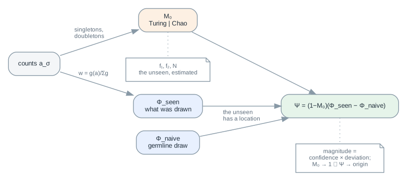
(2)#\[\Phi_{\text{true}} \;=\; (1 - M_0) \underbrace{\sum_{\text{seen}} \frac{p_\sigma}{\sum_{\text{seen}} p}\, z_\sigma}_{\Phi_{\text{seen}}} \;+\; M_0\, \mathbb{E}[z \mid \text{unseen}], \qquad M_0 = \sum_{\text{unseen}} p_\sigma .\]

This is an identity, not a model, and it is the unification: every weighting scheme in play is this one identity with a different estimator of \(M_0\). The current default is the special case \(M_0 = 0\) — the assumption that nothing was missed.

Two estimators of the missing mass #

Turing. \(\hat M_0 = f_1/N\): the classical read-weighted answer, the total frequency of clonotypes seen exactly once.

Chao, via a boundary assumption. Chao1 estimates the count of missing clonotypes and says nothing directly about their mass, so a bridge is needed. It is one assumption: an unseen clonotype is rare, so had it been drawn it would carry at most one read, and unseen clonotypes do not overlap. That pins each unseen clone’s frequency at the detection boundary \(1/(N + S_u)\), hence

\[\hat M_0 \;=\; S_u \cdot \frac{1}{N + S_u} \;=\; \frac{S_u}{N + S_u}, \qquad S_u \;=\; \frac{f_1(f_1-1)}{2(f_2+1)} ,\]

and substituting into (2) collapses the observed term to a single pseudo-count completion:

\[(1 - \hat M_0)\cdot \frac{a_\sigma}{N} \;=\; \frac{N}{N + S_u}\cdot\frac{a_\sigma}{N} \;=\; \frac{a_\sigma}{N + S_u} .\]

And this is why the units work. \(N\) counts reads while \(S_u\) counts clonotypes; adding them would normally be a category error, and is legitimate only because the one-read assumption makes each unseen clone contribute exactly one read — so \(N + S_u\) is the read total of the completed table. Read the formula as: sample slightly deeper, catch every missing clone exactly once.

Use the bias-corrected \(S_u = f_1(f_1-1)/(2(f_2+1))\), never the classical \(f_1^2/2f_2\): at these depths a sample with no clonotype seen exactly twice is common, and the classical form is undefined there. The two estimators rank samples nearly identically (measured \(r\) = 0.93 and 0.76 in two views) but differ in level — Chao runs above Turing when singletons dominate doubletons, below when doubletons abound. Both limits behave: a deep sample gives \(\hat M_0 = 0.0002\) and reduces to the ordinary embedding; an all-singleton sample gives 0.96, the honest statement that it measured almost nothing.

Sub-probability, not negative probability #

A natural question at this point is whether the missing mass could be a negative probability. It should not be, and it need not be. \(\Phi\)’s value is that \(\|\Phi_P - \Phi_Q\|\) is the MMD — a metric between distributions — and that a convex combination of two \(\Phi\)’s is the \(\Phi\) of a real pooled repertoire ((1)). A measure allowed to go negative on a set is not a probability measure: MMD stops being a metric on it, and the midpoint of two embeddings stops being the embedding of anything. Both losses are severe and neither is necessary.

Dropping the renormalisation instead costs nothing. Let the measure carry mass \(1 - M_0\):

\[\mu_S \;=\; \sum_{\text{seen}} w_\sigma\,\delta_{z_\sigma}, \qquad \text{total mass } = 1 - M_0 \;\le\; 1 .\]

Sub-probability measures are standard objects and nothing in the RKHS construction breaks. Interpretively this is the whole point: renormalising forces a 5-clonotype tumour to assert a full unit of confidence, whereas a deficient measure lets it say I hold 0.08 of a repertoire’s worth of evidence.

Where signed structure legitimately lives is a difference of two probability measures:

\[\Psi_S \;=\; (1 - M_0)\big(\Phi_{\text{seen}} - \Phi_{\text{naive}}\big) \;=\; \Phi_{\text{true}} - \Phi_{\text{naive}} ,\]

whose coordinates go negative wherever the sample is depleted relative to unselected V(D)J output — a real statement. It is an ordinary RKHS element and \(\|\Psi_S\|\) is exactly \(\mathrm{MMD}(S, \text{naive})\), so signed structure comes at no cost to the metric. The second equality is immediate from (2), and it is why the two constructions are one object rather than two: \(\Psi\) is the reference-centred sub-probability embedding.

Reading the result: magnitude = confidence × deviation-from-naive. An immune desert has \(M_0 \to 1\) and lands at the origin, the correct location for “no infiltrate detected” rather than an arbitrary point on the unit sphere. A vague, shallow blood sample lands there too and says so by its norm instead of by being dropped from the cohort.

Where the unseen lives #

One term in (2) is still unspecified, and it is not cosmetic: \(M_0\) alone only rescales \(\Phi\), so the unseen block changes the direction of the embedding only if it is actually filled with a vector. The choice of that vector decides whether the whole construction is a shrinkage estimator toward a meaningful point. Three candidates, measured:

prior for the unseen	verdict
the sample’s own singletons	begs the question — no new information enters
the corpus mean	James–Stein toward the centroid, and it measurably hurt: shallow samples pile into a dense ball that is itself depth-correlated
a germline draw	the one that works

Filling the unseen block with \(\sim 20{,}000\) naive V(D)J recombinations (mir.repertoire.naive_reference(), ~8 s) took \(R^2(\mathrm{PC}_1, \text{depth})\) from 0.259 to 0.001 in one view and 0.067 to 0.006 in another, with kNN label entropy unchanged or better. Checked against the degenerate explanation: the reference vector is finite, PC1’s explained variance was unchanged (0.309 → 0.334) so PC1 is a genuinely different direction rather than a collapsed one, and depth left the whole leading block (best of PC1–5: 0.253 → 0.047).

The mechanism is worth stating because it explains the failure above. \(\Phi = (1-M_0)\Phi_{\text{seen}} + M_0 z_{\text{naive}}\) is shrinkage: a shallow sample has large \(M_0\) and collapses toward a fixed point, a deep one keeps its own \(\Phi\). The difference from the failed James–Stein arm is entirely the target. Shrinking an unmeasurable sample toward the corpus centroid creates a dense ball that is itself depth-correlated; shrinking it toward the germline says the honest thing — a repertoire we did not measure looks like unselected recombination output — and lands it at a biologically meaningful location.

Call. sample_embedding(..., missing_mass="turing"|"chao") sets mass; mir.repertoire.missing_mass(), mir.repertoire.naive_reference(), mir.repertoire.contrast_embedding().

How much of a sample can be trusted #

The missing mass handled what was not seen. The other half of the sentence in When the sample is not a probability distribution was variance — and unlike bias, variance has a scale that can be estimated from the cohort itself.

The damage depth does to a kernel mean is not bias but variance \(\propto 1/n\), over an \(n\) spanning four orders of magnitude — and in a nearest-neighbour graph that heteroscedasticity is a depth axis, because a noisier point has systematically different neighbours. A 21-clonotype sample’s \(\Phi\) is \(\sim 16\times\) noisier than a 5,780-clonotype one’s. Measured, a sampling fingerprint (log reads, log unique, singleton fraction, Good–Turing missing mass, top-clone fraction) explained \(R^2 = 0.257\) of PC1 in one view and 0.465 in another.

Decompose the observed spread. Each sample’s squared distance from the cohort centroid has an expectation with two parts — real between-sample spread, plus sampling noise that shrinks with depth:

\[\mathbb{E}\big\|\Phi_S - \bar\Phi\big\|^2 \;\approx\; \underbrace{\tau^2}_{\text{signal}} \;+\; \underbrace{\frac{\sigma^2}{n}}_{\text{noise}}, \qquad \boxed{\;\kappa \;=\; \sigma^2/\tau^2\;}\]

so a straight line fitted to \(\|\Phi_S - \bar\Phi\|^2\) against \(1/n\) gives \(\tau^2\) as its intercept, \(\sigma^2\) as its slope, and \(\kappa\) as the sample size at which the two are equal. Below \(\kappa\), a sample’s \(\Phi\) is more sampling noise than signal.

Measured \(\kappa \approx 40\)–70 clonotypes across four independent views, with 23–69% of samples below it. The number is stable enough to be worth knowing and variable enough to be worth estimating rather than importing.

What to do with it is deliberately not “apply a floor”. The library applies none, because the same low clonotype count means opposite things in different tissues: in blood it is shallow sequencing, in a tumour it is low infiltration — the phenotype of interest. Measured, a floor applied in tumour deleted the stratum the analysis existed to predict. Carry \(\kappa\) and mass and weight instead of filtering; use \(\kappa\) to define the trusted subset a diagnostic is re-read inside, not to decide who is in the cohort.

Call. mir.repertoire.depth_threshold(), mir.repertoire.sample_statistics() / cohort_statistics() (the fingerprint), mir.cohort.depth_report() (R² of the leading PCs on the fingerprint, with a trusted-subset arm — read beside the returned explained_variance, which is what separates a different direction from a collapsed one).

The algebra that survives #

Mixture linearity (1) was established in step 2 and has been used once, to justify normalising. It licenses two further operations exactly — and “exactly” is what makes them worth having, because both would otherwise be heuristics.

Compartments and the dilution factor #

\(\Phi_1\) is a weighted average, which is the right operation for estimating a population mean and the wrong one for detecting a minority signal. Make that precise. Write the repertoire as naive plus expanded, \(\rho_S = (1-\pi)\rho_N + \pi\rho_E\); then by (1) a difference confined to the expanded compartment, \(\Delta = \Phi_1(E_{\text{case}}) - \Phi_1(E_{\text{ctrl}})\), reaches the whole-repertoire embedding attenuated to

\[\Phi_1(S_{\text{case}}) - \Phi_1(S_{\text{ctrl}}) \;=\; \pi\,\Delta ,\]

while the noise is supplied by the naive compartment, which contributes most of the clonotypes. The signal-to-noise ratio of the average is therefore worse than the compartment’s own by roughly \(\pi\) — and \(\pi\) is small precisely in the samples that matter. This is a statement about the estimator, not about the data, which is why it predicts a fix: embed the compartments separately.

Because (1) is exact, the shares are also recoverable after the fact by non-negative least squares — well-posed, not a heuristic fit:

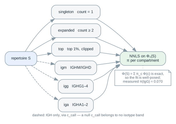
\[\hat\pi \;=\; \arg\min_{\pi \ge 0} \Big\| \Phi_1(S) - \sum_c \pi_c \Phi_1(c) \Big\|^2 .\]

Two implementation constraints follow from the mathematics rather than from taste. Every compartment must be embedded through the same basis — refitting per band would put each in its own geometry and make band-to-band and cohort-to-cohort distances meaningless. And a compartment with a handful of clonotypes is recorded absent, not embedded: a 3-clone “repertoire” is not an estimate, and a hole is a value the assembly layer already understands.

Measured on IGH isotypes, the class-switched IgG compartment carries a median \(\pi\) of 0.070 of \(\Phi_1(\text{IGH})\) (unswitched IgM 0.230, IgA 0.176, 0.520 unaccounted — the uncalled-isotype share, in ballpark agreement with the \(\sim 0.43\) counted from reads; embedding weight and reads are different denominators). Since IgG is the affinity-matured, T-dependent fraction most likely to carry antigen-specific signal, that single number is the dilution factor \(\pi\) measured rather than assumed — and it doubles as a power calculation: a subset carrying \(\pi \approx 0.001\) cannot be detected by any aggregate distance on \(\Phi\), so the per-clonotype witness (From vectors to answers) is the sensitive route. Check \(\pi\) before spending compute on the aggregate.

What the decomposition measured, in the direction the theory predicts: the singleton band reproduces a clinical-covariates-only score almost exactly (0.600 vs 0.599) — pure dilution — while expanded alone reproduces the whole-repertoire score (0.634 vs 0.634), so the entire prognostic content of \(\Phi_1\) lives in the expanded compartment. What it did not do is lift that content above what the clone-size distribution already encodes: on survival endpoints, zero of 22 pre-registered block × endpoint cells cleared the bar against a diversity reference, and the isotype cut failed identically. Where banding does win is where abundance classes are different biology — unmutated IgM singletons against class-switched expansions — with a measured kNN entropy of 0.3875 against 0.4686 for the pooled arm in tissue IGH.

Rarefaction, and the exact Rao gap #

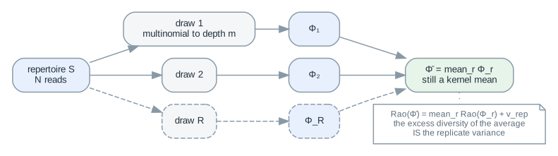
The second consequence answers “how do I compare two groups at matched depth without leaving the metric”. Because \(\Phi\) is linear in the measure, the mean of \(\Phi\) over \(R\) independent multinomial subsamples is itself a kernel mean embedding — of the mixture distribution over subsamples — so MMD, Rao and mixture linearity all survive (verified to \(\sim 10^{-15}\)). It is the only depth correction that does: an orthogonal projection breaks the norm identity, and a per-coordinate location-scale rescale breaks both.

The cost is also exactly computable, which is the appealing part. With \(\bar\Phi = R^{-1}\sum_r \Phi_r\) and \(v_{\text{rep}} = R^{-1}\sum_r \|\Phi_r - \bar\Phi\|^2\), the parallel-axis identity \(R^{-1}\sum_r\|\Phi_r\|^2 = \|\bar\Phi\|^2 + v_{\text{rep}}\) and \(Q = 1 - \|\Phi\|^2\) give

\[Q(\bar\Phi) \;=\; 1 - \|\bar\Phi\|^2 \;=\; 1 - \Big(\tfrac{1}{R}\!\sum_r \|\Phi_r\|^2 - v_{\text{rep}}\Big) \;=\; \frac{1}{R}\sum_r Q(\Phi_r) \;+\; v_{\text{rep}} .\]

Read it in either direction. As interpretation: \(\bar\Phi\) embeds the mixture over subsamples, which is genuinely more diverse than any single subsample, so the excess diversity of the average is the replicate variance. As a tool: \(v_{\text{rep}}\) is a free per-sample estimate of exactly the sampling noise that \(\kappa\) measures cohort-wide. And as a warning: averaging commutes with \(\Phi\) but not with nonlinear functionals of it, so \(\mathrm{mean}(Q) \ne Q(\mathrm{mean})\) and the gap must be reported rather than assumed away. Measured gaps ran 0.02% to 0.93%, monotone in target depth.

Rarefaction is not a default: rarefying a cohort to the depth of its shallowest useful samples discards the deep samples’ entire advantage. Reach for it when two groups must be compared at matched depth and the comparison has to stay an MMD.

Call. mir.repertoire.band_frames(), mir.repertoire.band_embeddings(), mir.repertoire.mixture_weights(), mir.repertoire.rarefy_embedding().

Back to the single clone: local density #

Everything so far aggregated the point cloud. The other question one can ask of the same points is local: is this receptor in a neighbourhood that is denser than chance? The kernel and its radius are already defined, so this needs no new geometry.

Enrichment as a density ratio #

Antigen-driven convergence appears as local over-density of receptors. Classical methods build an exact- or 1-mismatch sequence graph; the continuous form estimates the same ratio directly in embedding space (sec:dens-balloon, prop:balloon). With a balloon (adaptive-radius) estimator whose radius \(r(z)\) is chosen so the background ball holds a target count,

\[E(z) \;=\; \frac{\hat f_{\text{obs}}(z)}{\hat f_{\text{gen}}(z)} \;=\; \frac{n_{\text{obs}}(z)\,/\,N_{\text{obs}}}{n_{\text{gen}}(z)\,/\,N_{\text{gen}}} .\]

This is a density-ratio estimate (sec:dens-dre, lem:lsif), and the ratio form is what makes it usable in high \(p\): the ball volume cancels between numerator and denominator, so no bandwidth normalisation is needed and no density has to be estimated on its own — which in \(p\) of this size a kernel density estimate could not do. As \(r \to 0\) it recovers the graph limit, confirmed numerically (\(\rho\) 0.37 → −0.05 as the radius grows).

Two nulls, two background types #

The significance test depends on what the background is (prop:poissontest, prop:ctest):

\[n_{\text{obs}}(z) \sim \mathrm{Poisson}\big(\lambda(z)\big), \quad \lambda(z) = n_{\text{gen}}(z)\cdot \tfrac{N_{\text{obs}}}{N_{\text{gen}}} \qquad\text{(generative background)}\]

\[n_{\text{obs}}(z) \sim \mathrm{Binomial}\big(n_{\text{obs}}+n_{\text{gen}},\; p_0\big), \quad p_0 = \tfrac{N_{\text{obs}}}{N_{\text{obs}}+N_{\text{gen}}} \qquad\text{(control background)}\]

with Benjamini–Hochberg control across clonotypes, plus a water-level calibration (eq:waterlevel) that raises the null level until the empirical false-discovery profile is consistent — needed because in the naive regime the background is itself pervasively convergent.

That last point is the empirical lesson, and it matters more than the choice of test: real repertoires are so convergent that a generation-probability background flags \(\sim 40\%\) of clones. Use a biological control (day 15 versus day 0, allele-positive versus negative, seropositive versus control) for specificity, and process the full repertoire — subsampling dilutes exactly the sparse antigen clusters being looked for. Made quantitative on a spiked benchmark: admixed noise clones were over-flagged 43% under a generative background against 1% under a control background, a 46× signal-to-noise lift.

Abundance-aware enrichment #

Counting distinct neighbours ignores that an expanded clone is stronger evidence than a singleton (sec:dens-abund, prop:abund). Replace the in-ball count with the variance-stabilised mass \(S(z) = \sum_{j \in B(z)} g(a_j)\); under a compound-Poisson model its tail is Gamma with dispersion

\[\varphi \;=\; \frac{\mathbb{E}[g(A)^2]}{\mathbb{E}[g(A)]} ,\]

and a per-clonotype orphan/depth channel \(P(A \ge a_j)\) is Fisher-combined with the breadth term — so a clone can be called on being large where it should be small as well as on having many neighbours. Setting abundance=None recovers the distinct count exactly (\(g \equiv 1\)).

Call. mir.density.fit_density_space(), mir.density.neighbor_enrichment(), mir.density.enriched_mask(), mir.density.denoise_and_cluster(), mir.density.generate_background().

From vectors to answers #

A cohort is now a matrix of vectors. Two things are needed to report a result from it: a way to say which part of the vector carried the signal, and a correction for the nuisance structure that will otherwise carry it instead.

Named channels and ablation #

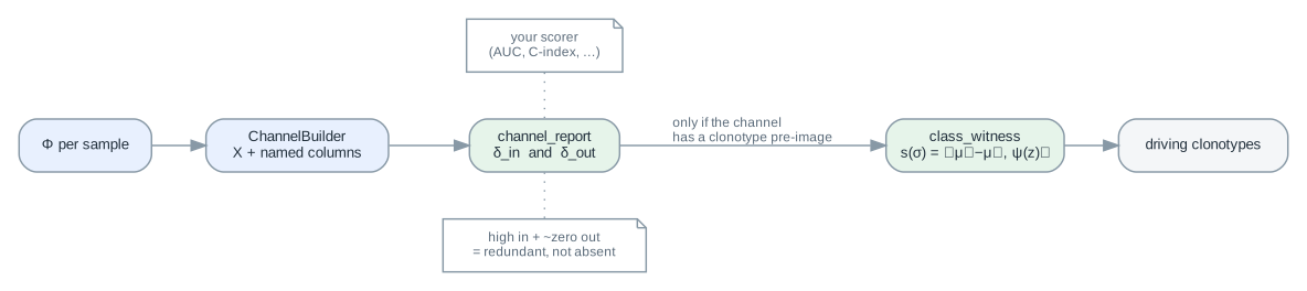
A channel is a named group of columns. Given a caller-supplied scorer \(f\) (higher is better) and a reference score \(b\), there are exactly two questions one can ask of a channel, and they are not the same question:

\[\delta_{\text{in}}(c) = f\big(X_{:,c}\big) - b, \qquad \delta_{\text{out}}(c) = f\big(X\big) - f\big(X_{:,\neg c}\big) .\]

\(\delta_{\text{in}}\) is marginal — inflated by correlation between channels, so two redundant channels both look important. \(\delta_{\text{out}}\) is conditional — deflated by the same correlation. Reported together they separate the claims: high in and high out means irreplaceable, while high in with \(\delta_{\text{out}} \approx 0\) is the redundancy signature. Leave-one-in is the default for a concrete reason: real scorers reduce their input (an in-fold PCA), so dropping one narrow channel lets the reduction re-mix the rest and reconstruct nearly the same components, making leave-one-out structurally near-blind to exactly the 1-column channels that often win.

Significance, when asked for, is a row permutation of the block: the scorer holds \(y\) in row order, so shuffling the block’s rows breaks the association exactly as shuffling \(y\) would, and it is the only null available to a function that never sees the labels.

The witness: from a difference back to sequences #

An MMD between two groups is a number; the witness function turns it back into receptors (prop:witness, eq:witness). The direction \(\mu_{\text{pos}} - \mu_{\text{neg}}\) in feature space scores each candidate clonotype by

\[s(\sigma) \;=\; \big\langle \mu_{\text{pos}} - \mu_{\text{neg}},\; \psi(\varphi(\sigma)) \big\rangle ,\]

so the top-scoring candidates are the discriminative public clones. This is the supervised route to motifs that the unsupervised bulk mean cannot surface, because there they are swamped by the naive background — the same dilution argument as Compartments and the dilution factor, which is why a small \(\pi\) sends you here.

Note what can and cannot be attributed this way. Only a channel with a clonotype pre-image — a kernel mean — has a witness; a Hill number is a summary of the count distribution and has no pre-image, so asking which clones drive it is a category error rather than a hard problem.

Batch offsets, and why the obvious correction backfires #

A first-order batch effect is an additive offset, so subtracting each batch’s mean removes it (prop:batch) — in-sample. Out-of-sample the estimation error dominates. With \(\hat\mu_b\) fitted from \(n_b\) samples in \(d\) dimensions,

\[\mathbb{E}\|\hat\mu_b - \mu_b\|^2 \;=\; \frac{\sigma^2 d}{n_b} ,\]

which for \(n_b \approx 8\)–15 and \(d \approx 1{,}280\) is a vector of norm \(\approx 16\) against a true offset of norm 7–24: subtracting it injects a batch-constant vector as large as the one it removes. Measured, evaluated leave-one-batch-out plus a donor-level split inside each batch, batch-identity AUC went 0.863 raw → 0.985 after per-batch centring and 0.978 after ComBat. Both classical corrections made the batch easier to read.

The fix is to shrink the offset by its own reliability. The positive-part James–Stein estimator,

\[\hat\mu_b^{\text{JS}} \;=\; c_b\,\hat\mu_b, \qquad c_b \;=\; \Big(1 - \frac{(d-2)\,\hat\sigma^2/n_b}{\|\hat\mu_b\|^2}\Big)_+ ,\]

leaves alone any batch whose apparent offset is no larger than its estimation error, and measured, it recovered most of the damage: 0.985 → 0.889. The cluster-aware alternative removes the offset per soft cluster with a batch-diversity penalty (Harmony-style), which corrects a batch confounded with biology instead of erasing that biology, and reduces exactly to plain residualisation at one cluster.

Three conditions any correction must meet, learned the hard way: evaluate out-of-sample, since in-sample the injected error is invisible by construction; report the geometry cost (within-batch distance correlation, idempotence, symmetry) and not only the batch metric; and check mixture additivity (1), because the compartment decompositions depend on it.

Call. mir.explain.ChannelBuilder, mir.explain.channel_report(), mir.explain.channel_drivers(), mir.repertoire.class_witness(), mir.cohort.residualize() (shrink=True for the James–Stein form), mir.repertoire.correct_batch(), and the scorers in mir.bench.eval.

From vectors back to biology #

The construction so far is one-directional: a repertoire in, a vector out. The remaining question is whether the arrow can be reversed — whether a point in the space can be turned back into a repertoire state, a trajectory, or a sequence.

The derivable descriptor #

\(\Phi\) normalises the total mass away, and in tissue that mass is the infiltration signal. The descriptor keeps it as a coordinate (rem:descriptor):

\[\mathrm{desc}(S) \;=\; \Big(\underbrace{\log\textstyle\sum_\sigma a_\sigma}_{\text{infiltration}},\; \underbrace{-\log \textstyle\sum_\sigma w_\sigma^2}_{\log n_{\text{eff}}},\; \underbrace{\textstyle\sum_\sigma w_\sigma^2}_{\text{clonality}},\; \underbrace{\Phi_1(S)}_{\text{identity}}\Big) .\]

Every coordinate is smooth — no integer richness — and every named metric is readable back off the vector analytically. Smoothness is the requirement that makes the object simulatable: fit a density over a cohort’s descriptors and the coordinate distribution is a generative manifold rather than a scatter of labels.

In-silico evolution #

Fit a (optionally class-conditional) Gaussian \(\mathcal{N}(m,\Sigma)\) with Ledoit–Wolf shrinkage over descriptor vectors. Then “perturb one coordinate and let the rest follow” is not a heuristic but the Gaussian conditional mean (prop:evolve): splitting into the perturbed coordinate \(1\) and the rest \(2\),

\[\mathbb{E}\big[x_2 \mid x_1 = m_1 + \delta\big] \;=\; m_2 + \Sigma_{21}\Sigma_{11}^{-1}\,\delta ,\]

so “make this donor hotter” propagates through every coupled coordinate using the cohort’s own covariance. Measured couplings match immunobiology: hotter ⇒ diversity \(+0.84\), class-switch \(+0.52\), T-versus-B \(-0.63\). The non-linear alternative is a compact conditional DDPM/DDIM over the same descriptor space with classifier-free guidance, sharing the sample(n, condition=…) call shape so either generator drops in unchanged.

Covariate-disentangled trajectory #

A cohort often has a known covariate (allele, batch, arm) and an unknown progression axis (days since exposure, severity). The PhenoPath-style model (eq:phenopath, prop:trajectory-fit) infers the latter while separating out which channels respond to it differently by covariate:

\[Y_{ng} \;=\; c_g \;+\; \alpha_g^\top x_n \;+\; \big(\kappa_g + \gamma_g^\top x_n\big)\,\tau_n \;+\; \varepsilon_{ng} ,\]

with \(\tau_n\) the trajectory position of sample \(n\), \(\kappa_g\) a channel’s baseline response, and \(\gamma_g\) the covariate × trajectory interaction — the term that answers “does this channel move differently in carriers”. Fitting alternates closed-form per-channel ridge regressions with a GLS update for \(\tau\),

\[\tau_n \;=\; \frac{\sum_g \beta_{ng}\,\big(Y_{ng} - c_g - \alpha_g^\top x_n\big)/s_g^2} {\sum_g \beta_{ng}^2/s_g^2}, \qquad \beta_{ng} = \kappa_g + \gamma_g^\top x_n ,\]

with ARD-style iteratively-reweighted shrinkage on \(\gamma\) (rem:phenopath-approx; a simplified closed-form approximation to PhenoPath’s CAVI inference, not a reimplementation of it).

Sequence reconstruction #

The last arrow to reverse is step 1. The junction embedding is compressible: PCA retaining 95% of the variance suffices for geometry (clustering, MMD), while reconstruction needs 99% — the chain-adaptive lesson. A codec learns \(\text{seq} \to \text{code} \to \text{seq}\) with a geometry anchor, so the code stays near the true embedding instead of drifting to whatever is easiest to decode:

\[\mathcal{L} \;=\; \underbrace{\mathcal{L}_{\text{recon}}}_{\text{token cross-entropy}} \;+\; \lambda_{\text{embed}}\,\underbrace{\big\|\,\text{code} - \text{PCA}(\varphi(\sigma))\,\big\|^2} _{\text{distances preserved}} .\]

Reconstruction turned out to be training-data-limited, not architecture-limited: the same one-shot decoder goes from exact-match 0.885 at \(n = 20`k to 0.941 at 50k to 0.958 at 100k. Levers in order: more data (free) > more PCs (to ~99% variance) > :math:`K \to \sim 2000\) (it saturates; \(K = 10{,}000\) regresses) > an autoregressive decoder for the last percent.

Note the direction of information flow before using this. The distance-to-prototypes code is an expansion (\(\sim 10\) kbit against a \(\sim 63\)-bit sequence), so for archival losslessness one stores the string; the codec inverse exists for ML and generation — decoding a synthetic point that no observed clonotype occupies. And as in step 1, embeddings are comparable only if the prototype panel and the PCA rotation match, which is why a codec ships as a bundle carrying both plus a prototype hash, and refuses to load against a different panel.

Call. mir.repertoire.sample_descriptor(), mir.generate.DescriptorDensity, mir.twin.DonorTwin, mir.ml.diffusion, mir.track.fit_exposure_trajectory(), mir.ml.codec, mir.ml.bundle.

The contract: which transformation preserves what #

Each of the three steps bought a property, and each property licensed a class of operation. The practical consequence is that no transformation of \(\Phi\) is neutral: it keeps some and breaks others, and which ones decides what may still be computed downstream.

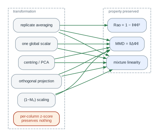
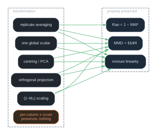
transformation	MMD \(=\\|\Delta\Phi\\|\)	Rao \(=1-\\|\Phi\\|^2\)	mixture linearity	use
replicate averaging (rarefaction)	✔	✔ (with the exact \(v_{\text{rep}}\) gap)	✔	matched-depth comparison
global scalar rescale	✔ (up to scale)	✘	✔	magnitude-carrying blocks
centring / PCA projection	✔	✘	✔ (affine, same shift per band)	visualisation, Cox input
per-column standardisation	✘	✘	✘	never on a magnitude block
orthogonal projection	✔ (on the retained subspace)	✘	✔	nuisance removal
sub-probability scaling \((1-M_0)\)	✔ (as a signed contrast)	✘	✔	deficient coverage

Two rows deserve to be read twice.

Per-column standardisation. It forces every coordinate to unit variance across samples, so a matrix in which half the rows sit at the origin comes out looking exactly like one in which none do — it deletes the deficiency it was meant to preserve. This already invalidated one experiment, whose deficient arm scored 0.6481 against a 0.6179 baseline purely from the rescaling. Any block whose point is that magnitude carries information must be scaled by one global scalar: ChannelBuilder.add(..., preserve_magnitude=True).

Centring. It keeps differences and therefore MMD, but not norms — so Rao’s \(Q\) cannot be read off a centred or PCA-reduced identity block, and any norm-based quantity has to be recomputed from the true \(\Phi_1\). A related trap follows from step 1’s all-positive coordinates: the shared profile puts any two TCREmp-derived vectors at raw cosine \(\approx 0.999\), and subtracting each vector’s own scalar mean does not fix it (measured: 0.9993 raw, 0.9985 self-centred, \(-0.14\) cohort-centred). Only cohort centring removes the shared profile, so read a cosine between two such vectors only after it.

Where to go next #

The spine of this page was: coordinates (Step 1 — a sequence becomes a point) → a well-defined object (Step 2 — a sample becomes a measure) → a comparable vector (Step 3 — a measure becomes a vector) → what it contains (What the vector already knows) → the premise that fails and its repair (When the sample is not a probability distribution, How much of a sample can be trusted) → what the surviving algebra licenses (The algebra that survives) → the three directions out (Back to the single clone: local density, From vectors to answers, From vectors back to biology) → what may be done to \(\Phi\) at all (The contract: which transformation preserves what).

For the full derivations, the theory appendix of the companion manuscript is the reference, and the labels used in parentheses throughout this page are its labels. For the empirical record — which arm won, on which cohort, with which interval — see the benchmark documents in the companion analysis repository. For the calls themselves, each section ends with them, and the API reference has the signatures.