User guide

One task per section, cheapest-to-run first. Every embedding operates on polars frames keyed by the AIRR column names v_call / j_call / junction_aa (and duplicate_count for clone sizes). Sections build on each other but each is self-contained.

Install & the data model

pip install mirpy-lib            # core: import mir, and the `mir` CLI
pip install "mirpy-lib[bench]"   # + benchmark harness (matplotlib, huggingface_hub, lifelines)
pip install "mirpy-lib[ann]"     # + approximate-NN density backend (pynndescent)
pip install "mirpy-lib[ml]"      # + neural codecs (torch)
pip install "mirpy-lib[examples]"# + marimo notebooks (marimo, matplotlib, umap-learn)

Requires vdjtools>=3.0.0 and seqtree>=0.3.0; mir itself is a pure-Python py3-none-any wheel. A clonotype table is a polars frame; clone sizes live in duplicate_count (repertoire-level embeddings weight by them):

import polars as pl

sample = pl.DataFrame({
    "v_call":          ["TRBV10-3*01",   "TRBV20-1*01",   "TRBV28*01"],
    "j_call":          ["TRBJ2-7*01",    "TRBJ1-2*01",    "TRBJ2-1*01"],
    "junction_aa":     ["CASSIRSSYEQYF", "CSARVSGYYGYTF", "CASSLGQAYEQFF"],
    "duplicate_count": [120,             40,              12],
})

To read a file in any format instead, use vdjtools.io.read (AIRR TSV, vdjtools, MiXCR, immunoSEQ, parquet — the format is sniffed): sample = vdjtools.io.read("sample.tsv").

Clonotype embedding

TCREmp maps each clonotype to a fixed vector — the concatenation of its distances to a set of prototype clonotypes, per component (V, J, junction). Distance in this space approximates the pairwise alignment distance (Theory T1).

from mir.embedding.tcremp import TCREmp

model = TCREmp.from_defaults("human", "TRB", n_prototypes=1000)
X = model.embed(sample)                  # (3 rows, 3×1000) float32, interleaved [v, j, junction]

# paired chains: a dict of per-locus frames -> concatenated embedding
from mir.embedding.tcremp import PairedTCREmp
paired = PairedTCREmp.from_defaults("human", ("TRA", "TRB"))
Xp = paired.embed({"TRA": tra_df, "TRB": trb_df})

Which prototypes?

The prototype set is the coordinate system, so it is worth one paragraph. mirpy bundles 10 000 real receptors per chain — a uniform random sample (fixed seed=42) of unique, productive, germline-resolvable clonotypes from arda-annotated real repertoires, for human TRA/TRB/TRG/TRD/ IGH/IGK/IGL and mouse TRA/TRB. Real, not model-generated: synthetic P_gen junctions have degenerate lengths and embed measurably worse. Nothing is downloaded at import or build time; provenance and the regenerate command are in SOURCES.md.

replicate=0 — the first n rows — is the prototype set: what every preset, bundled codec and published number uses. To ask “is my result an artefact of which prototypes I drew?”, take a replicate. The file order is itself a uniform shuffle, so each disjoint block of n rows is an independent draw from the same pool — n_replicates() of them, 10 at n=1000, 5 at n=2000:

from mir.embedding.prototypes import n_replicates, load_prototypes

n_replicates("human", "TRB", 1000)                      # -> 10
scores = [my_metric(TCREmp.from_defaults("human", "TRB", 1000, replicate=r).embed(sample))
          for r in range(10)]                           # spread = prototype-draw sensitivity

Usually it matters very little, and prototype_source_correlation() measures it directly — it correlates the pairwise junction-distance geometry under two prototype sets, so handing it two replicates answers the question at the geometry level. On 400 held-out human-TRB queries, two independent draws agree at R = 0.922 (n=100), 0.971 (250), 0.990 (500), 0.993 (1000, the default), 0.997 (2000): from n≈500 up the geometry is effectively draw-independent, and only below n≈250 does the particular draw start to show.

Warning

Each replicate is a different coordinate system. Distances within one are comparable, distances across two are not — the prototype hash covers the replicate index, so RepertoireSpace, DonorCohort and the codec bundles all refuse to mix them. Compare summary statistics across replicates, never raw embeddings. Sweeping n_prototypes is a different question: those draws are nested (r=0 at n=500 is a prefix of n=1000), so a sweep answers “how many do I need”, not “does it matter which”.

Pick prototype counts / PCA dims from the per-chain presets, and denoise with PCA:

from mir.embedding.presets import get_preset
from mir.embedding.pca import pca_denoise

preset = get_preset("human", "TRB")      # n_prototypes, n_components (95% var), recon dims
Xd = pca_denoise(X, n_components=preset.n_components)

From the shell — the mir embed clonotypes command does exactly this on a file:

mir embed clonotypes sample.tsv --pca 50 -o clonotypes.parquet
#   input:  any format vdjtools.io reads; locus inferred (or pass --locus)
#   output: one row per clonotype (id columns + e0…), TSV or (recommended for the wide raw
#           embedding) Parquet.  --n-prototypes / --mode / --pca / --threads for the knobs.

Clustering antigen-specific TCRs

Antigen-specific receptors form tight clusters in the embedding. mir.bench clusters them and scores per-antigen F1 / retention against known labels (e.g. a VDJdb dump):

from mir.bench.metrics import cluster, cluster_metrics

labels = cluster(pca_denoise(X, n_components=50), method="dbscan")   # or "hdbscan" / "optics"
# with epitope labels aligned to the rows:
metrics = cluster_metrics(labels, epitopes)                         # {epitope: AntigenMetric}

DBSCAN (default) is tightest/purest; HDBSCAN trades precision for ~3× coverage on variable-density data. See examples/quickstart.py for the end-to-end VDJdb example with a UMAP.

Density and background subtraction

mir.density finds antigen-driven convergent clusters by neighbour enrichment in the embedding space (graph-free TCRNET/ALICE, Theory T6): E(z) = f_obs(z) / f_gen(z) estimated by an adaptive-bandwidth balloon estimator with a Poisson/binomial test and BH q-values.

from mir.density import fit_density_space, neighbor_enrichment, enriched_mask, denoise_and_cluster

# background = a biological control (TCRNET) or generate_background(...) (ALICE, P_gen)
space, obs_emb, bg_emb = fit_density_space(model, obs_df, control_df, n_components=20)
res  = neighbor_enrichment(obs_emb, bg_emb, test="binomial")   # exact multicore kdtree by default
hits = obs_df.filter(enriched_mask(res, alpha=0.05))           # background-subtracted clones
labels, mask = denoise_and_cluster(obs_emb, res)               # noise-filter + cluster the hits

Prefer a biological control (e.g. pre/post-vaccination) over the P_gen background — differential enrichment cancels generic public convergence and isolates the antigen-specific response. Without one of your own, pooled healthy-donor repertoires are a single hf_hub_download away (isalgo/airr_control, read with vdjtools.io.read; see SOURCES.md), and generate_background() remains the P_gen fallback — pass source="arda" when the observed data is arda-annotated (one allele namespace, no cascade fallback) and species="mouse" for mouse. The neighbour engine defaults to backend="kdtree" (exact, multicore); at whole-repertoire scale pass backend="ann" (approximate, [ann] extra). See examples/density.py.

Repertoire embedding Φ(S) + MMD

mir.repertoire embeds a whole repertoire — an order-invariant multiset of clonotypes with clone sizes — into one fixed vector Φ(S) (kernel mean ‖ Hill diversity ‖ second moment), depth-robust into the RNA-seq regime (Theory T7). Every sample in a cohort must share one basis, fit once:

from mir.repertoire import (fit_repertoire_space, sample_embedding,
                            mmd_matrix, hla_stratified_mmd, class_witness)
import polars as pl

space = fit_repertoire_space(model, pl.concat(samples))    # ONE basis for the cohort
embs  = [sample_embedding(space, s) for s in samples]      # Φ(S); each .vector is the tensor
D     = mmd_matrix(embs, unbiased=True)                    # pairwise MMD (unbiased when depth varies)

# supervised motif finder: public clones separating two groups
motifs = class_witness(space, pos_samples, neg_samples, candidates)

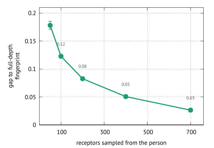
Read only a few hundred receptors and Φ is already close to the full-depth fingerprint — the gap shrinks as n_eff^{-1/2} (Theory prop:kme):

Use unbiased=True whenever samples differ in depth/diversity — the biased V-statistic’s 1/n_eff self-term otherwise inflates low-diversity samples and fakes a signal. For a batch-confounded contrast, compare within-batch (residualise Φ on the batch indicator, see the cohort section): a batch offset is first-order and cancels, while a batch-orthogonal signal (e.g. HLA) survives.

From the shell — mir embed repertoires fits one shared basis per chain and writes the Φ table:

mir embed repertoires cohort/*.tsv.gz -o phi.tsv --mmd mmd.tsv
#   one input file per repertoire (sample id = filename stem); one output row per sample per
#   chain (sample_id, locus, n_clonotypes, phi0…). --blocks mean,diversity[,second] and
#   --weight / --n-rff pick the Φ layout;  --mmd also writes the pairwise unbiased-MMD matrix.

Multi-chain digital donor (mir.cohort)

mir.cohort fuses per-chain repertoire embeddings into one digital donor matrix — an identity (kernel-mean) block plus diversity and coverage channels, per locus, merged by name. The result is hash-verified (the prototypes and the fitted PCA must match) and serialisable, so a held-out donor is projected through the same basis:

from mir.repertoire import fit_repertoire_spaces, correct_batch
from mir.cohort import fit_donor_embeddings, residualize, cluster_samples

spaces = fit_repertoire_spaces(models, cohort_frames)        # one RepertoireSpace per locus
cohort = fit_donor_embeddings(spaces, donor_frames)          # DonorCohort{X, spec, ...}
cohort.save("cohort.npz")                                    # carries every locus' prototype hash

Xc  = residualize(cohort.X, batch)                           # first-order: subtract each batch mean
Xc  = correct_batch(cohort.X, batch)                         # Harmony-like cluster-aware, when the
                                                             # batch is confounded with biology (T7 prop:batch)
lab = cluster_samples(embs, unbiased=True)                   # MMD-cluster repertoires into states

residualize removes a global batch offset; correct_batch removes it per soft cluster (reducing to residualize at n_clusters=1), so a batch confounded with a biological cluster is corrected without erasing that biology.

Explainable channel readout (mir.explain)

Φ.vector is an anonymous concatenation, so “the classifier found something” has no noun. mir.explain attaches the names and asks which of them carries the signal. The scorer is yours — the library never sees the labels, so the same call serves a cross-validated AUC or a Cox C-index (scorers live in mir.bench.eval):

from mir.explain import stack_embeddings, channel_report
from mir.bench.eval import cv_auc

X, spec = stack_embeddings(embs)                     # X[i] is exactly embs[i].vector; names attached
rep = channel_report(X, spec, lambda B: cv_auc(B, y)[0], base=0.5)
rep.best                                             # -> 'second'  (the HLA imprint lives here)
rep.frame()                                          # channel | n_columns | score | delta | rank

Leave-one-in (the default) asks whether a channel carries the signal alone; it is marginal, so correlated channels both look important. mode="both" adds the conditional half — a channel with a high delta but delta_out ≈ 0 is redundant, its signal duplicated elsewhere. Assemble heterogeneous channels (per-chain blocks merge by name) with ChannelBuilder, and mark the kernel-mean blocks attributable so the readout can go one hop further, to the clones:

from mir.explain import ChannelBuilder, channel_drivers
from mir.bench.eval import cv_cindex

b = ChannelBuilder()
for c in chains:
    b.add("identity", ident[c], attributable=True).add("diversity", hill[c])
X, spec = b.add("coverage", log_reads).build()      # median-impute + z-score
rep = channel_report(X, spec,
                     lambda B: cv_cindex(dur, evt, base=clin, block=B, n_pc=8),
                     base=cv_cindex(dur, evt, base=clin), mode="both")

channel_drivers(rep, space=space, pos=pos, neg=neg, candidates=cands)

Only a kernel-mean channel has a clonotype pre-image. Asking which clones drive a Hill number is a category error, and channel_drivers raises rather than answer it.

Survival / classification scorers (mir.bench.eval)

The scorers the readout consumes are plain functions of a feature block and your labels — usable on their own:

from mir.bench.eval import cv_auc, cv_cindex, km_logrank

mean, std = cv_auc(X, y)                             # repeated stratified-CV AUC (mean, std)
c = cv_cindex(dur, evt, base=clin, block=X, n_pc=8)  # Cox C-index of clinical covariates + X
c0 = cv_cindex(dur, evt, base=clin)                  # …the base to compare it against
p = km_logrank(dur, evt, groups)                     # multivariate log-rank p-value

Needs the [bench] extra (scikit-learn is core; cv_cindex / km_logrank use lifelines).

Neural codecs (mir.ml)

The optional mir.ml tier ([ml] extra, torch) trains fast neural approximations of the embedding: a forward encoder (sequence → code), an inverse decoder (code → sequence), a Pgen regressor, and a unified codec; plus a learned repertoire set encoder. Device selection is automatic (CUDA → MPS → CPU; override with device= or MIR_DEVICE).

from mir.ml.bundle import CodecBundle

bundle = CodecBundle.load("path/to/codec")
encoder = bundle.forward_encoder()           # refuses a prototype-hash mismatch
codes = encoder.code(sample["junction_aa"].to_list())     # CDR3 strings -> compact codes
emb = encoder.encode(sample["junction_aa"].to_list())     # …or the full-space embedding

Training scripts and shipped bundles live in the companion analysis repo; this tier is experimental.

Benchmark harness & reproducing the paper

mir.bench provides the VDJdb clustering benchmark (F1 / retention / purity) and the reproduced theory experiments (S1–S3, T5–T6, codec losslessness). The self-contained theory runs on bundled data via examples/theory.py; the full benchmark suite lives in the 2026-mirpy-analysis repo.

from mir.bench.vdjdb import load_vdjdb, antigen_subset
from mir.bench.metrics import cluster, cluster_metrics

df = antigen_subset(load_vdjdb("vdjdb.slim.txt.gz"), chain="TRB", min_records=30)
X = model.embed(df)                                   # df is already AIRR-named
labels = cluster(pca_denoise(X, n_components=50))
metrics = cluster_metrics(labels, df["epitope"])      # {epitope: AntigenMetric}