Figure gallery

Every panel below is one call to tcren.viz.pymol.render() on a scene from the same module, ray-traced by a headless PyMOL. They are library functions rather than notebook snippets, so a figure in a paper, in a notebook and in a script are the same figure.

pip install "tcren[viz]"     # matplotlib + py3Dmol; PyMOL itself is a separate install
tcren fetch-data             # populates data/Canonical2026

Reading the axis gizmo

Every panel carries a thin, arrow-headed triad in its bottom-left corner. A canonically-oriented structure is not interpretable unless the reader can tell which way the frame points, and x/y/z does not tell them, so the arrows are named for what they mean:

axis	label	direction
x	width	groove width, across the cleft (α1↔α2)
y	N→C	groove axis, signed toward the peptide C-terminus
z	TCR	docking normal, MHC floor → TCR

The triad turns with the camera. An axis pointing at the viewer foreshortens to a dot, and its label drops to the lower left of that dot — the usual convention for an axis normal to the page. So in a top-down view TCR sits at the origin, and in a side-on view N→C does.

These are the three directions the docking-geometry literature uses; the principal-component ranking differs from it because tcren.orient.frame fits the whole complex where the groove-only conventions fit the MHC alone. tcren.viz.pymol.CANONICAL_AXES carries the names, the definitions and the correspondence.

The peptide in the groove

Looking down the docking normal, from where the TCR sits: the peptide as sticks in the cleft, the MHC coloured by domain — helices salmon, β-sheet floor cyan.

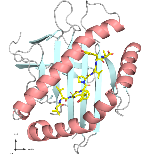
from tcren.viz.pymol import render, groove_scene
render(groove_scene("1ao7", "data/Canonical2026"), "groove.png")

With surface=True the MHC gains a translucent molecular surface, which is how histo.fyi presents a structure — the cleft reads as a cleft rather than as ribbon.

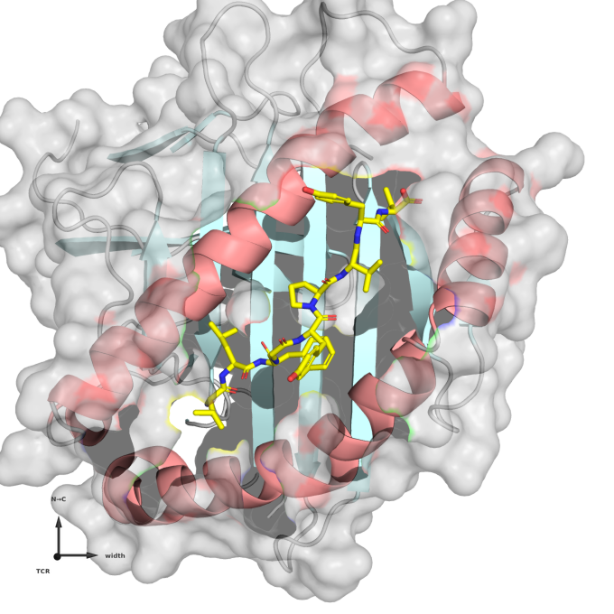
render(groove_scene("1ao7", "data/Canonical2026", surface=True), "surface.png")

Which residues carry the score

The interface energy Φ is a sum over residue–residue contacts, so it decomposes exactly: each residue’s share is the sum of φ(a_i, a_j) over the contacts it makes across the interface. That is the quantity worth colouring by — the total says how large the score is, the decomposition says what it is made of.

tcren.viz.pymol.residue_importance() computes it and tcren.viz.pymol.importance_scene() paints it: CDR3 and peptide residues as sticks on a ramp, everything else pale.

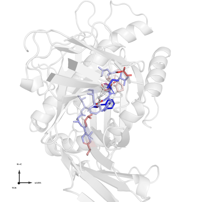
from tcren.viz.pymol import render, residue_importance, importance_scene

imp = residue_importance(structure)          # per-residue phi and contact count
render(importance_scene("1ao7", "data/Canonical2026", imp), "importance.png")

Blue is favourable, red unfavourable. The ramp is centred on zero rather than fitted to the observed range, so the colours keep that meaning: a range-fitted ramp would paint the least-favourable residue red even in an interface where every contact is stabilising.

The same call colours by the geometric share instead — how much of the interface a residue physically occupies, rather than how much energy it contributes. A residue can be large on one and small on the other, and that difference is usually the interesting part.

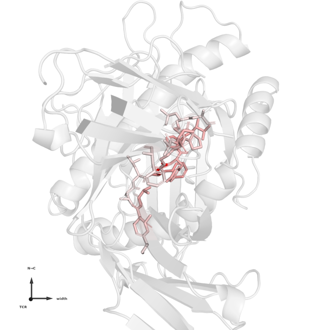
render(importance_scene("1ao7", "data/Canonical2026", imp,
                        by="n_contacts", spectrum="white_red"), "contacts.png")

Note

Each contact is attributed to both residues it joins, so the per-residue values sum to twice Φ. It is an attribution, not a partition — the energy of a contact belongs to the pair, not to either partner.

The recognition interface

Peptide plus the CDR1–3 loops that reach it, over a pale MHC, seen side-on — the plane the crossing and incident angles live in.

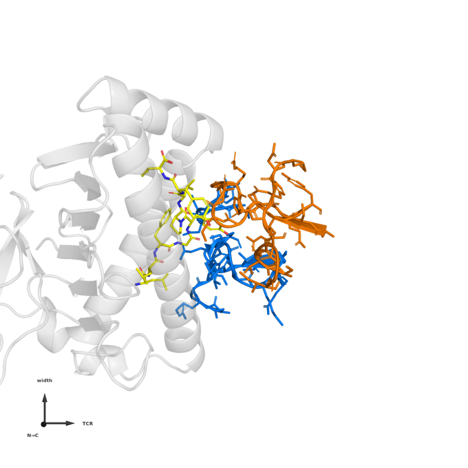
from tcren.viz.pymol import render, interface_scene
render(interface_scene("1ao7", "data/Canonical2026", cdr_resi), "interface.png")

An ensemble in one frame

Because orientation puts every structure in the same frame, an overlay is meaningful: the MHC superposes and the spread you see is real variation in how the receptors dock.

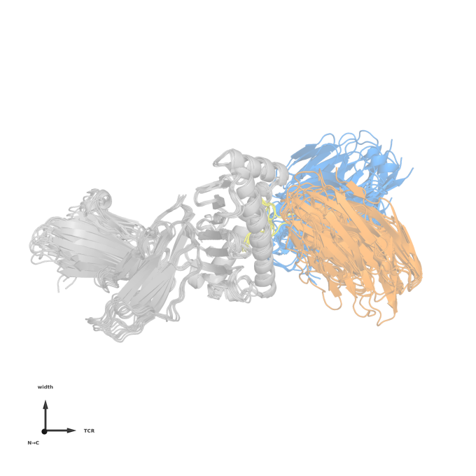
from tcren.viz.pymol import render, overlay_scene
render(overlay_scene(pdb_ids, "data/Canonical2026"), "overlay.png")

Exploring interactively

Two notebooks in notebooks/ drive all of the above:

pymol_canonical_figures.ipynb

The static gallery — every view family over the four MHC class × species groups.

pymol_interactive.py

A marimo app: pick a structure and a scene, swing the camera and watch the gizmo follow, restyle it, and rotate a live 3Dmol.js view with the mouse.

pip install marimo
marimo run notebooks/pymol_interactive.py     # or `marimo edit` to change the code

For a viewer inside a Jupyter notebook without leaving Python, tcren.viz.view_pocket_cdr() returns a py3Dmol view of the same oriented groove.