2D complementarity maps

Project the TCR-peptide-MHC interface (CDR1-3, peptide, MHC groove helices/floor) onto the canonical groove plane, build the two canonical polars tables (residue markup + contacts), and render a metadata-rich SVG complementarity map.

# Environment versions (reproducibility)
import sys, polars as pl, tcren
print('python', sys.version.split()[0], '| polars', pl.__version__, '| tcren', tcren.__version__)

python 3.11.15 | polars 1.41.2 | tcren 0.1.0

# Load a native complex, type chains (arda) and annotate the MHC groove
from tcren.structure import parse_structure
from tcren.annotation import classify_chains
from tcren.mhc import annotate_mhc

structure = parse_structure('data/Native2026/1ao7.pdb.gz', pdb_id='1ao7')
classify_chains(structure, organism='human')
annotate_mhc(structure)
[(c.chain_id, c.chain_type) for c in structure.chains]

[('A', 'TRA'), ('B', 'TRB'), ('C', 'PEPTIDE'), ('D', 'MHCa'), ('E', 'B2M')]

# Project onto the canonical groove plane and build the canonical tables
from tcren.project2d import (project_structure, residue_markup_table,
                             contacts_table, ca_contacts_table, pocket_markers)

projection = project_structure(structure)
markup = residue_markup_table(structure, projection)
contacts = contacts_table(structure, threshold=5.0)
ca_contacts = ca_contacts_table(structure, threshold=8.0)
pockets = pocket_markers(markup)
markup.head()

shape: (5, 14)

structure_id	structure_chain	complex_chain	complex_region	residue_index	aa_index	aa_len	aa	x	y	z	u	v	height
str	str	str	str	i64	i64	i64	str	f64	f64	f64	f64	f64	f64
"1ao7"	"A"	"tra"	"fr1"	1	0	110	"K"	null	null	null	null	null	null
"1ao7"	"A"	"tra"	"fr1"	2	1	110	"E"	null	null	null	null	null	null
"1ao7"	"A"	"tra"	"fr1"	3	2	110	"V"	null	null	null	null	null	null
"1ao7"	"A"	"tra"	"fr1"	4	3	110	"E"	null	null	null	null	null	null
"1ao7"	"A"	"tra"	"fr1"	5	4	110	"Q"	null	null	null	null	null	null

# Contacts table is compatible with the original TCRen 5 A calculation
contacts.head()

shape: (5, 11)

structure_id	structure_chain_1	structure_chain_2	residue_index_1	residue_index_2	aa_index_1	aa_index_2	min_dist	contact_type	backbone_1	backbone_2
str	str	str	i64	i64	i64	i64	f64	str	bool	bool
"1ao7"	"D"	"E"	235	10	234	9	2.447153	"hydrogen_bond"	true	false
"1ao7"	"A"	"C"	31	5	30	4	2.54217	"hydrogen_bond"	false	false
"1ao7"	"C"	"D"	1	171	0	170	2.631378	"hydrogen_bond"	true	false
"1ao7"	"A"	"B"	50	105	49	100	2.63158	"hydrogen_bond"	false	false
"1ao7"	"A"	"B"	35	106	34	101	2.647912	"hydrogen_bond"	false	true

# Render the SVG complementarity map (squares=residues, bold=Ca-Ca, dashed=inter-residue)
from tcren.viz import render_complementarity_map
from IPython.display import SVG

svg = render_complementarity_map(markup, contacts=contacts, ca_contacts=ca_contacts, pockets=pockets)
SVG(svg)

Multiple views of the same complex

The full map above shows the whole interface. Below are focused complementarity-map views (chain subsets — the TCR↔peptide footprint, and the peptide sitting in the MHC groove) followed by three orthogonal structural views of the oriented complex. Contacts in every view are the same closest-atom edges read off the contact table.

# Different complementarity-map VIEWS via chain subsets (edges = contacts read off the map).
from IPython.display import display
map_views = {'TCR (CDR1-3) ↔ peptide': ['tra', 'trb', 'peptide'],
             'peptide in the MHC groove': ['peptide', 'mhca', 'mhcb']}
for title, chains in map_views.items():
    print(title)
    display(SVG(render_complementarity_map(
        markup, contacts=contacts, ca_contacts=ca_contacts, pockets=pockets, show_chains=chains)))

TCR (CDR1-3) ↔ peptide

peptide in the MHC groove

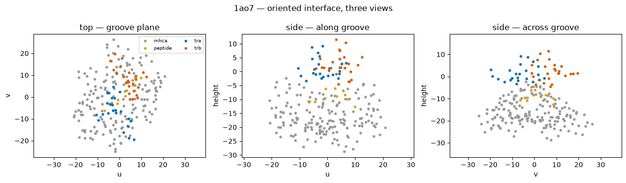
# Different STRUCTURAL views: the oriented interface in 3 orthogonal planes.
# u = along the groove (peptide N->C), v = across the groove, height = MHC->TCR normal.
# The canonical frame puts the TCR on top (+height) of the peptide/MHC.
import matplotlib.pyplot as plt
m = markup.filter(pl.col('u').is_not_null())
chain_col = {'mhca': '#999999', 'mhcb': '#777777', 'peptide': '#E69F00',
             'tra': '#0072B2', 'trb': '#D55E00'}
planes = [('u', 'v', 'top — groove plane'),
          ('u', 'height', 'side — along groove'),
          ('v', 'height', 'side — across groove')]
fig, axes = plt.subplots(1, 3, figsize=(13, 3.8))
for ax, (a1, a2, ttl) in zip(axes, planes):
    for ch, col in chain_col.items():
        sub = m.filter(pl.col('complex_chain') == ch)
        if sub.height:
            ax.scatter(sub[a1], sub[a2], s=16, c=col, label=ch, edgecolor='none')
    ax.set_xlabel(a1); ax.set_ylabel(a2); ax.set_title(ttl); ax.set_aspect('equal', 'datalim')
axes[0].legend(fontsize=7, ncol=2, loc='best')
fig.suptitle('1ao7 — oriented interface, three views'); plt.tight_layout(); plt.show()

# Polars summarize: contact-type breakdown of the TCR (CDR) -> peptide interface
tcr_pep = (contacts
    .join(markup.select('structure_chain', 'aa_index', 'complex_chain', 'complex_region'),
          left_on=['structure_chain_1', 'aa_index_1'],
          right_on=['structure_chain', 'aa_index'])
    .filter(pl.col('complex_chain').is_in(['tra', 'trb'])
            & pl.col('structure_chain_2').is_in([c.chain_id for c in structure.chains if c.chain_type=='PEPTIDE'])))
tcr_pep.group_by('complex_region', 'contact_type').agg(
    pl.len().alias('n'), pl.col('min_dist').min().round(2).alias('closest')
).sort('complex_region', 'n', descending=[False, True])

shape: (6, 4)

complex_region	contact_type	n	closest
str	str	u32	f64
"cdr1"	"hydrogen_bond"	4	2.54
"cdr1"	"polar"	3	3.66
"cdr1"	"hydrophobic"	1	4.93
"cdr3"	"polar"	13	3.32
"cdr3"	"hydrophobic"	4	3.66
"cdr3"	"hydrogen_bond"	4	2.89