PyMOL renders of canonically-oriented TCR–pMHC complexes#
Publication-ready ray-traced panels of the Canonical2026 set (HF isalgo/tcren_structures, oriented by tcren orient), over the four MHC class × species groups.
Every render is driven by ``tcren.viz.pymol`` — the scenes, the styling and the axis gizmo are library code with unit tests, so a figure here and a figure made from a script are the same figure. This notebook only chooses what to draw.
The axis gizmo#
Each panel carries a thin, arrow-headed triad in its bottom-left corner, turning with the camera. An oriented structure is only interpretable if the reader can tell which way the frame points, and x/y/z does not tell them — so the arrows are named for what they mean:
axis |
label |
what it is |
|---|---|---|
x |
|
groove width, across the cleft (α1↔α2) |
y |
|
the groove axis, toward the peptide C-terminus |
z |
|
the docking normal, MHC floor → TCR |
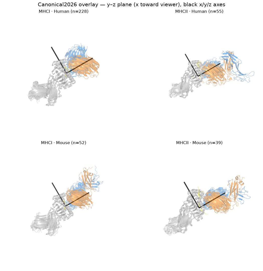
An axis pointing at the viewer foreshortens to a dot, and its label falls to the lower left of that dot — the usual convention for an axis normal to the page. So in the side views N→C sits at the origin, and in the top-down views TCR does.
These are the same three directions the docking-geometry literature uses (SwiftTCR, TCR3d); only the principal-component ranking differs, because tcren.orient.frame fits the whole complex while those fit the MHC groove alone.
Chain roles after orientation: A=Vα, B=Vβ, C=peptide, D=MHCα, E=MHCβ/β2m.
[1]:
# Setup: group the oriented structures by MHC class x species. All rendering comes from the library.
import json, collections
from pathlib import Path
import matplotlib.pyplot as plt, matplotlib.image as mpimg

from tcren.viz.pymol import (CANONICAL_AXES, render, overlay_scene, groove_scene,
                             interface_scene)

CANON = Path('../data/Canonical2026')   # repo-root data/ (notebook cwd is notebooks/)
OUT = Path('/tmp/tcren_figs'); OUT.mkdir(exist_ok=True)
GROUPS = [('MHCI', 'Human'), ('MHCII', 'Human'), ('MHCI', 'Mouse'), ('MHCII', 'Mouse')]

meta = [r for r in json.load(open('../src/tcren/data/orient_metadata.json')) if r.get('status') == 'ok']
by_group = collections.defaultdict(list)
for r in meta:
    if (CANON / f"{r['pdb.id']}.pdb.gz").exists():
        by_group[(r['mhc.class'], r['species'])].append(r['pdb.id'])
print({g: len(by_group[g]) for g in GROUPS})

# The frame every panel's gizmo reports, straight from the library so this cannot drift.
for a in CANONICAL_AXES:
    print(f"  {a.letter} -> {a.short:6s} {a.label:14s} {a.definition}")

def panel(pngs, titles, suptitle):
    # Assemble rendered PNGs into one figure. Each PNG already carries its own axis gizmo.
    fig, ax = plt.subplots(2, 2, figsize=(11, 11))
    for a, p, t in zip(ax.ravel(), pngs, titles):
        a.imshow(mpimg.imread(p)); a.set_title(t, fontsize=12); a.axis('off')
    fig.suptitle(suptitle, fontsize=15); plt.tight_layout(); plt.show()
{('MHCI', 'Human'): 228, ('MHCII', 'Human'): 55, ('MHCI', 'Mouse'): 52, ('MHCII', 'Mouse'): 39}
  x -> width  groove width   PC3, the thin axis; across the cleft, α1↔α2 helix separation
  y -> N→C    peptide N→C    PC2, the groove/peptide axis, signed toward the peptide C-terminus
  z -> TCR    pMHC→TCR       PC1, the MHC→TCR long axis, signed toward the TCR; the MHC sits at −z
1. Overlay in canonical coordinates — side-on (overlay_scene)#
[2]:
# Up to 8 structures per group, superposed, seen side-on: the image plane is the groove axis by
# the docking normal, which is the plane the crossing and incident angles live in.
pngs = [render(overlay_scene(by_group[g], CANON), OUT / f'ov_{g[0]}_{g[1]}.png', size=(900, 900))
        for g in GROUPS]
panel(pngs, [f'{c} · {s} (n={len(by_group[(c, s)])})' for c, s in GROUPS],
      'Canonical2026 overlay — side-on; N→C points at the viewer')
2. Top-down: peptide sticks in the MHC groove (groove_scene)#
[3]:
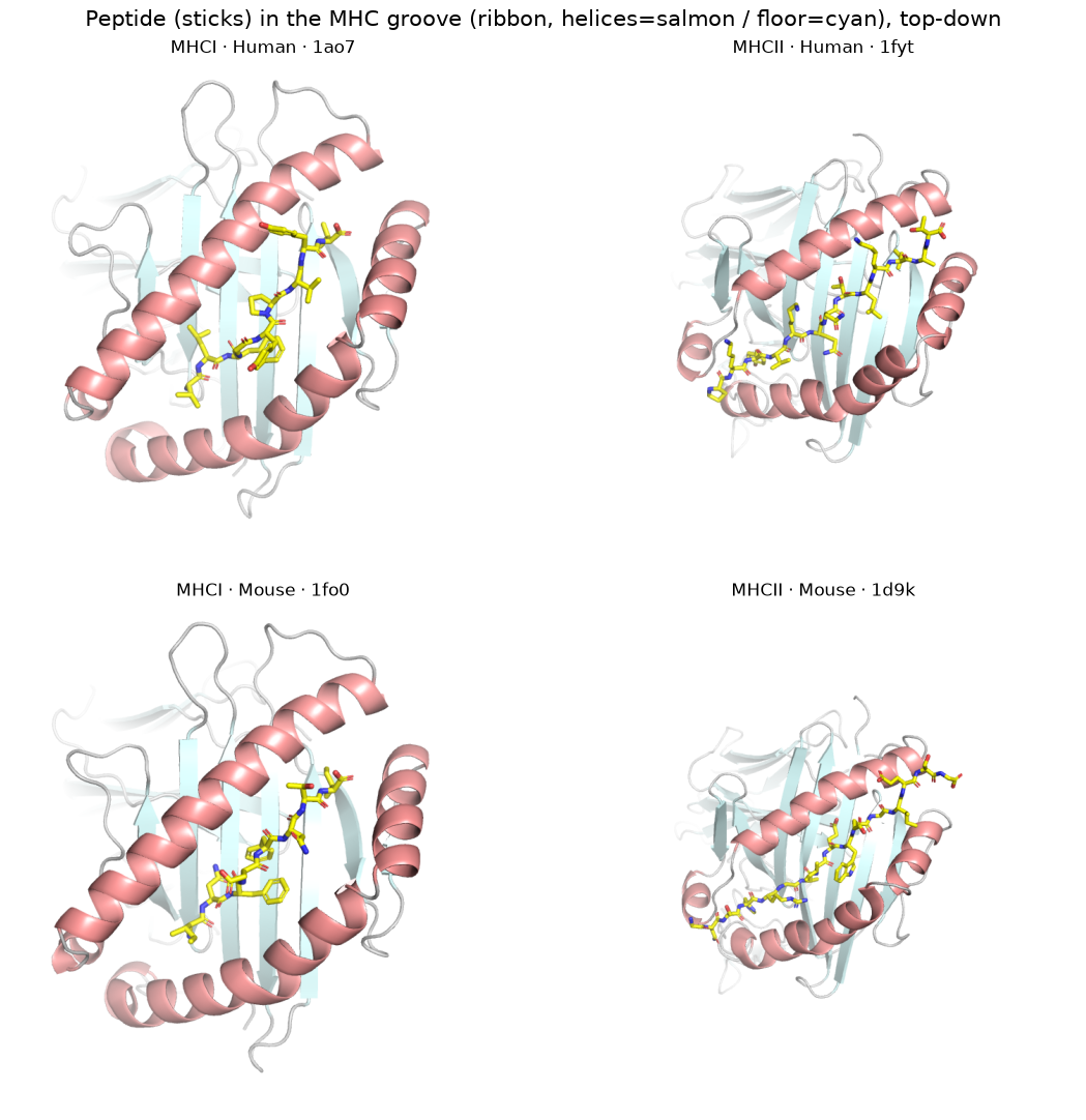
# One representative per group, looking down the docking normal from where the TCR sits:
# the peptide as sticks in the cleft, the MHC coloured by domain (helices vs beta-sheet floor).
pngs = [render(groove_scene(by_group[g][0], CANON), OUT / f'gr_{g[0]}_{g[1]}.png', size=(900, 900))
        for g in GROUPS]
panel(pngs, [f'{c} · {s} · {by_group[(c, s)][0]}' for c, s in GROUPS],
      'Peptide in the MHC groove, top-down (helices salmon / floor cyan); TCR points at the viewer')
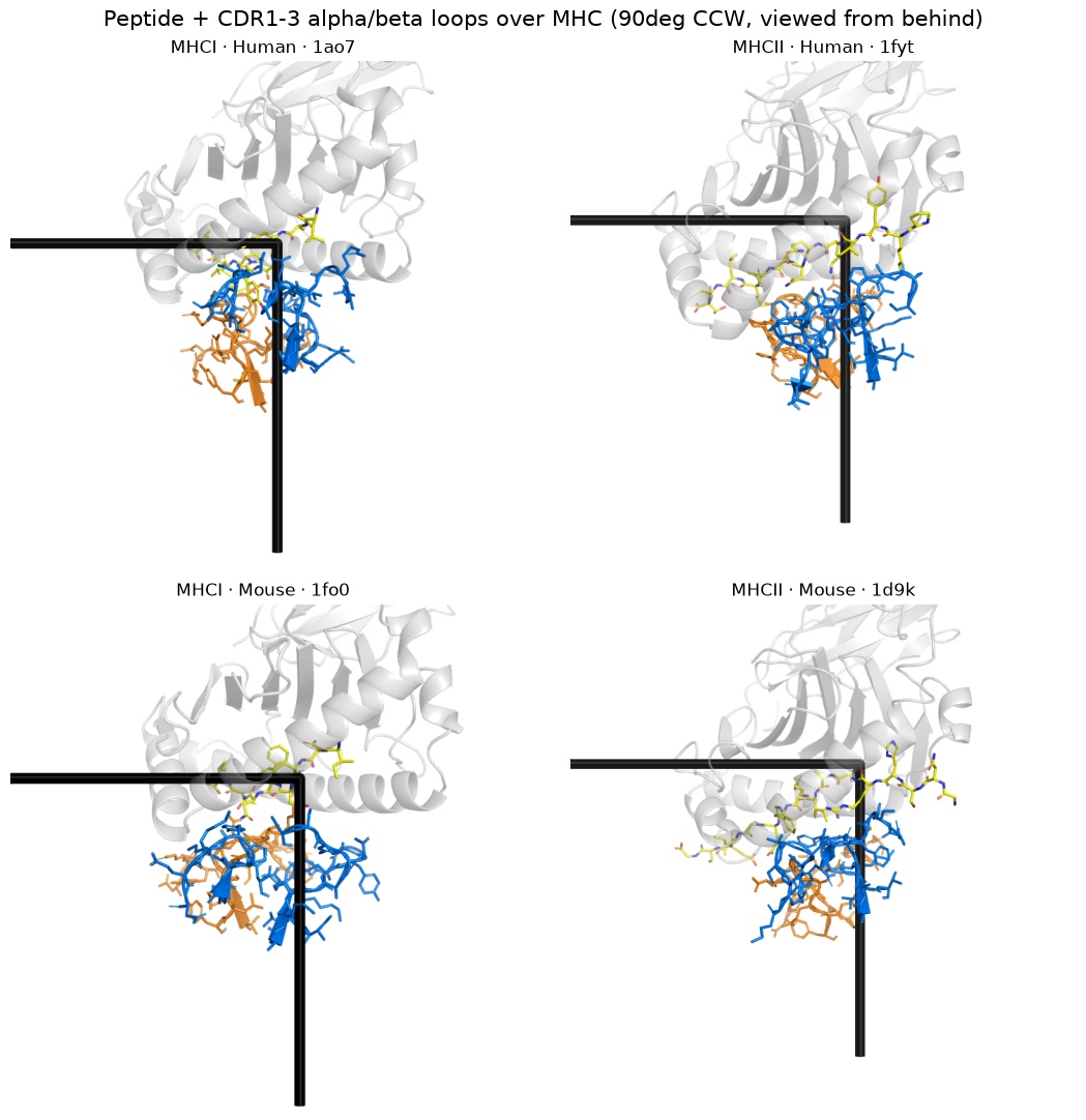
3. Interface: peptide + CDR1–3 α/β loops over the MHC (interface_scene)#
[4]:
# CDR residues come from annotating the pre-orientation Native2026 structure; PDB numbering
# survives orientation, so the same numbers select chain A/B (=TRA/TRB) in the oriented file.
import warnings; warnings.filterwarnings('ignore')
from tcren.structure import import_structure
from tcren.annotation import classify_chains

def cdr_resi(pid):
    s = import_structure(f'../data/Native2026/{pid}.pdb.gz', pdb_id=pid)
    classify_chains(s, organism='human')
    out = {'TRA': [], 'TRB': []}
    for c in s.chains:
        if c.chain_type in out:
            for reg in c.regions:
                if reg.region_type.startswith('CDR'):
                    out[c.chain_type] += [r.pdb_index for r in reg.residues]
    return out

pngs = [render(interface_scene(by_group[g][0], CANON, cdr_resi(by_group[g][0])),
               OUT / f'if_{g[0]}_{g[1]}.png', size=(900, 900)) for g in GROUPS]
panel(pngs, [f'{c} · {s} · {by_group[(c, s)][0]}' for c, s in GROUPS],
      'Peptide + CDR1–3 α/β loops over the MHC, side-on')
4. Surface view, histo.fyi-style (e.g. 5tez)#
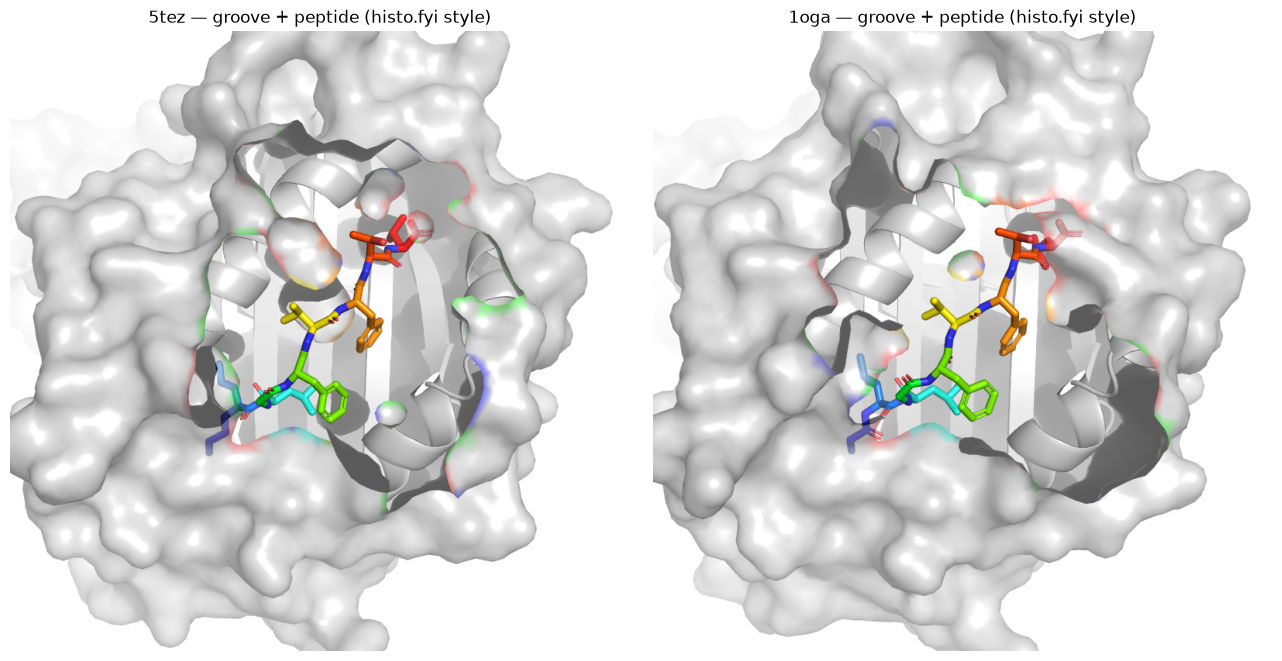
A clean look into the peptide-binding groove: the MHC as a pale translucent surface over its ribbon, the peptide as sticks threaded along the cleft, on white. Same scene as §2 with surface=True.
[5]:
# The same groove scene with the molecular surface on, which is how histo.fyi presents a structure:
# a pale MHC with the peptide threaded along the cleft. `surface=True` is the only change.
ex = [p for p in ('5tez', '1oga') if (CANON / f'{p}.pdb.gz').exists()] or [by_group[('MHCI', 'Human')][0]]
pngs = [render(groove_scene(p, CANON, surface=True), OUT / f'hf_{p}.png', size=(1000, 1000))
        for p in ex]
fig, ax = plt.subplots(1, len(pngs), figsize=(6.5 * len(pngs), 6.5), squeeze=False)
for a, p, pid in zip(ax.ravel(), pngs, ex):
    a.imshow(mpimg.imread(p)); a.set_title(f'{pid} — groove + peptide, surface on'); a.axis('off')
plt.tight_layout(); plt.show()