VDJBet YF Analysis (Rmd-aligned)#
Python rewrite of tmp/vdjbet_snippet.Rmd with matching analysis outputs:
YF vs OLGA V-usage and V/J correction factors
LLW reference and adjusted mock generation
LLW Pgen histogram match against mock bins
LLW overlap per sample: matched clonotypes and duplicate_count
Cohen d, z-scores, empirical p-values, FDR
Red line (LLW) + mock boxplots and Cohen d heatmaps
[1]:
# Remove stale control locks left by killed processes before any control builds.
import os, signal
from pathlib import Path

_locks_dir = Path.home() / '.cache' / 'mirpy' / 'controls' / '.locks'
if _locks_dir.exists():
    for _lf in sorted(_locks_dir.glob('*.lock')):
        try:
            _pid = int(_lf.read_text().split('pid=')[1].split()[0])
            try:
                os.kill(_pid, 0)   # process still alive — keep lock
            except (ProcessLookupError, PermissionError):
                _lf.unlink(missing_ok=True)
                print(f'Removed stale lock: {_lf.name} (pid={_pid} dead)')
        except Exception:
            pass
print('Lock check done.')
Lock check done.
[2]:
import importlib.metadata as _meta
import sys as _sys
print(f"Python {_sys.version.split()[0]}")
for _pkg in ["mirpy-lib", "numpy", "pandas", "matplotlib", "scipy", "polars"]:
    try:
        print(f"  {_pkg}: {_meta.version(_pkg)}")
    except _meta.PackageNotFoundError:
        pass

import math
import sys
import warnings
from collections import Counter
from pathlib import Path

import matplotlib.pyplot as plt
import numpy as np
import pandas as pd

repo_root = Path.cwd().resolve().parent if Path.cwd().name == "notebooks" else Path.cwd().resolve()
if str(repo_root) not in sys.path:
    sys.path.insert(0, str(repo_root))

from mir.comparative.vdjbet_workflow import (
    bh_fdr,
    build_real_control_analysis,
    build_synthetic_comparison,
    compute_bin_alignment_diagnostics,
    compute_olga_usage_adjustment,
    load_yfv_trb_samples,
    score_samples_dataframe,
)
from mir.common.parser import load_vdjdb_latest
from mir.utils.notebook_assets import ensure_airr_yfv19, notebook_large_assets_root

SEED = 42
N_MOCKS = 1000
POOL_SIZE = 100_000
OLGA_USAGE_N = 1_000_000
# count_rearrangement (default, unweighted) or count_duplicates (weighted by duplicate_count)
USAGE_COUNT_MODE = "count_rearrangement"
USAGE_PSEUDOCOUNT = 1.0
YFV_CACHE_DIRNAME = "pkl_trb_repertoires"

ASSET_ROOT = notebook_large_assets_root(repo_root)
YFV_DIR = ensure_airr_yfv19(repo_root)

print(f"YFV_DIR = {YFV_DIR}")
print(f"ASSET_ROOT = {ASSET_ROOT}")
print(f"Usage mode = {USAGE_COUNT_MODE}, pseudocount = {USAGE_PSEUDOCOUNT}")
print(f"OLGA usage cache size = {OLGA_USAGE_N:,}")
print(f"N_MOCKS = {N_MOCKS}")

# Publication-quality matplotlib style (Nature/Science aesthetics)
plt.rcParams.update({
    "font.family": "sans-serif",
    "font.sans-serif": ["Arial", "Helvetica", "DejaVu Sans"],
    "font.size": 10,
    "axes.titlesize": 11,
    "axes.labelsize": 10,
    "xtick.labelsize": 9,
    "ytick.labelsize": 9,
    "legend.fontsize": 9,
    "figure.dpi": 150,
    "savefig.dpi": 300,
    "axes.linewidth": 0.8,
    "axes.spines.top": False,
    "axes.spines.right": False,
    "xtick.major.size": 3.5,
    "ytick.major.size": 3.5,
    "xtick.direction": "out",
    "ytick.direction": "out",
    "axes.grid": False,
})
Python 3.12.12
  mirpy-lib: 1.1.0
  numpy: 1.26.4
  pandas: 3.0.3
  matplotlib: 3.10.9
  scipy: 1.17.1
  polars: 1.40.1
/Users/mikesh/vcs/mirpy/.venv/lib/python3.12/site-packages/tqdm/auto.py:21: TqdmWarning: IProgress not found. Please update jupyter and ipywidgets. See https://ipywidgets.readthedocs.io/en/stable/user_install.html
  from .autonotebook import tqdm as notebook_tqdm
YFV_DIR = /Users/mikesh/vcs/mirpy/notebooks/assets/large/airr_yfv19
ASSET_ROOT = /Users/mikesh/vcs/mirpy/notebooks/assets/large
Usage mode = count_rearrangement, pseudocount = 1.0
OLGA usage cache size = 1,000,000
N_MOCKS = 1000
1. Load LLWNGPMAV TRB reference from VDJdb#
[3]:
vdjdb_rep = load_vdjdb_latest(
    epitope="LLWNGPMAV",
    locus="TRB",
    species="HomoSapiens",
    mhc_a_contains="A*02",
)
print(f"Reference clonotypes: {vdjdb_rep.clonotype_count}")
if vdjdb_rep.clonotype_count > 0:
    print(f"Example: {vdjdb_rep.clonotypes[0].junction_aa}  {vdjdb_rep.clonotypes[0].v_gene}  {vdjdb_rep.clonotypes[0].j_gene}")
else:
    print("Warning: no clonotypes returned for this epitope/allele in VDJdb. Downstream cells may fail.")
Downloading: https://github.com/antigenomics/vdjdb-db/releases/download/2026-05-16/vdjdb-2026-05-16.zip
LLWNGPMAV: 409 unique TRB clonotypes
Reference clonotypes: 409
Example: CAIQDAGASYEQYF  TRBV6-2*01  TRBJ2-7*01
2. Load YF samples#
[4]:
# Load YF TRB repertoires and build per-sample records for VDJBet.
warnings.filterwarnings("ignore", category=FutureWarning)

samples, yfv_gu = load_yfv_trb_samples(YFV_DIR)

print(f"Loaded TRB samples: {len(samples)}")
print(f"Total TRB clonotypes: {sum(s['repertoire'].clonotype_count for s in samples):,}")
print(f"Total TRB duplicates: {sum(s['repertoire'].duplicate_count for s in samples):,}")
Loaded TRB samples: 42
Total TRB clonotypes: 29,939,151
Total TRB duplicates: 56,732,204
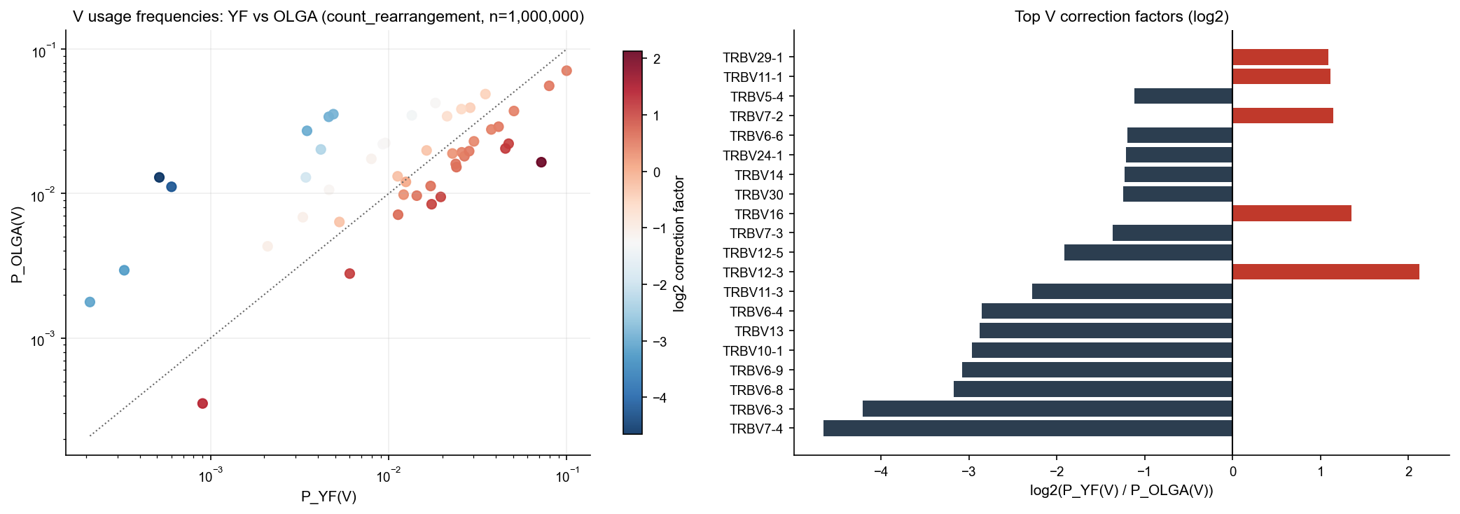
3. OLGA usage and correction factors#
Compute OLGA and YF usage frequencies, then derive correction factors.
Frequencies are computed in GeneUsage with configurable count mode and Laplace smoothing:
mode count_rearrangement: count of unique clonotypes per key / total clonotypes
mode count_duplicates: sum duplicate_count per key / total duplicate_count
pseudocount 1 is added for both YF and OLGA sides
Formulas:
factor_v = P_YF(V) / P_OLGA(V)
factor_vj = P_YF(V,J) / P_OLGA(V,J)
These factors are used by PgenGeneUsageAdjustment.
[5]:
usage_result = compute_olga_usage_adjustment(
    yfv_gu,
    seed=SEED,
    n_jobs=8,
    olga_usage_n=OLGA_USAGE_N,
    count_mode=USAGE_COUNT_MODE,
    pseudocount=USAGE_PSEUDOCOUNT,
)

olga_model = usage_result.olga_model
olga_gu = usage_result.olga_usage
v_cmp = usage_result.v_cmp
vj_cmp = usage_result.vj_cmp
v_df = usage_result.v_df
if hasattr(v_df, "to_pandas"): v_df = v_df.to_pandas()
vj_df = usage_result.vj_df
if hasattr(vj_df, "to_pandas"): vj_df = vj_df.to_pandas()

# Keep OLGA-based adjustment for the synthetic-null comparison section.
pgen_adj_olga = usage_result.pgen_adj_olga

print("Top V genes by |log2 factor|:")
display(v_df.assign(abs_log2=lambda d: d["log2_factor_v"].abs()).sort_values("abs_log2", ascending=False).head(15))
print("Top VJ pairs by |log2 factor|:")
display(vj_df.assign(abs_log2=lambda d: d["log2_factor_vj"].abs()).sort_values("abs_log2", ascending=False).head(15))

fig, axes = plt.subplots(1, 2, figsize=(14, 5))

x = np.clip(v_df["p_yf"].values, 1e-12, None)
y = np.clip(v_df["p_olga"].values, 1e-12, None)
sc = axes[0].scatter(x, y, c=v_df["log2_factor_v"].values, cmap="RdBu_r", s=40, alpha=0.9)
axes[0].plot([x.min(), x.max()], [x.min(), x.max()], color="#666666", linestyle=":", linewidth=1)
axes[0].set_xscale("log")
axes[0].set_yscale("log")
axes[0].set_xlabel("P_YF(V)")
axes[0].set_ylabel("P_OLGA(V)")
axes[0].set_title(f"V usage frequencies: YF vs OLGA ({USAGE_COUNT_MODE}, n={OLGA_USAGE_N:,})")
axes[0].grid(alpha=0.2)
cb = plt.colorbar(sc, ax=axes[0], shrink=0.9)
cb.set_label("log2 correction factor")

top = v_df.assign(abs_log2=lambda d: d["log2_factor_v"].abs()).sort_values("abs_log2", ascending=False).head(20)
axes[1].barh(top["v_gene"], top["log2_factor_v"], color=["#c0392b" if z > 0 else "#2c3e50" for z in top["log2_factor_v"]])
axes[1].axvline(0, color="black", linewidth=1)
axes[1].set_title("Top V correction factors (log2)")
axes[1].set_xlabel("log2(P_YF(V) / P_OLGA(V))")

plt.tight_layout()
plt.show()

print(f"Zero-frequency OLGA V genes in comparison table: {(v_df['p_olga'] == 0).sum()}")
Top V genes by |log2 factor|:
| v_gene | p_yf | p_olga | factor_v | log2_factor_v | abs_log2 | |
|---|---|---|---|---|---|---|
| 42 | TRBV7-4 | 0.000514 | 0.012933 | 0.039769 | -4.652226 | 4.652226 |
| 34 | TRBV6-3 | 0.000602 | 0.011130 | 0.054079 | -4.208799 | 4.208799 |
| 38 | TRBV6-8 | 0.000327 | 0.002943 | 0.111047 | -3.170758 | 3.170758 |
| 39 | TRBV6-9 | 0.000210 | 0.001774 | 0.118152 | -3.081285 | 3.081285 |
| 0 | TRBV10-1 | 0.003474 | 0.027168 | 0.127878 | -2.967164 | 2.967164 |
| 9 | TRBV13 | 0.004602 | 0.033953 | 0.135543 | -2.883182 | 2.883182 |
| 35 | TRBV6-4 | 0.004885 | 0.035428 | 0.137887 | -2.858442 | 2.858442 |
| 5 | TRBV11-3 | 0.004155 | 0.020195 | 0.205763 | -2.280945 | 2.280945 |
| 6 | TRBV12-3 | 0.071966 | 0.016474 | 4.368434 | 2.127116 | 2.127116 |
| 8 | TRBV12-5 | 0.003422 | 0.012931 | 0.264602 | -1.918104 | 1.918104 |
| 41 | TRBV7-3 | 0.013478 | 0.034757 | 0.387772 | -1.366720 | 1.366720 |
| 12 | TRBV16 | 0.000900 | 0.000352 | 2.557484 | 1.354725 | 1.354725 |
| 23 | TRBV30 | 0.009252 | 0.021960 | 0.421335 | -1.246962 | 1.246962 |
| 10 | TRBV14 | 0.009560 | 0.022397 | 0.426836 | -1.228247 | 1.228247 |
| 17 | TRBV24-1 | 0.018288 | 0.042331 | 0.432027 | -1.210806 | 1.210806 |
Top VJ pairs by |log2 factor|:
| v_gene | j_gene | p_yf | p_olga | factor_vj | log2_factor_vj | abs_log2 | |
|---|---|---|---|---|---|---|---|
| 565 | TRBV7-4 | TRBJ1-2 | 0.000024 | 0.001272 | 0.018877 | -5.727231 | 5.727231 |
| 71 | TRBV11-3 | TRBJ1-5 | 0.000054 | 0.002093 | 0.025665 | -5.284056 | 5.284056 |
| 575 | TRBV7-4 | TRBJ2-6 | 0.000006 | 0.000204 | 0.027196 | -5.200448 | 5.200448 |
| 564 | TRBV7-4 | TRBJ1-1 | 0.000040 | 0.001453 | 0.027859 | -5.165700 | 5.165700 |
| 473 | TRBV6-4 | TRBJ1-3 | 0.000030 | 0.001063 | 0.028051 | -5.155828 | 5.155828 |
| 474 | TRBV6-4 | TRBJ1-4 | 0.000049 | 0.001615 | 0.030113 | -5.053479 | 5.053479 |
| 567 | TRBV7-4 | TRBJ1-4 | 0.000019 | 0.000608 | 0.030893 | -5.016563 | 5.016563 |
| 462 | TRBV6-3 | TRBJ1-5 | 0.000039 | 0.001222 | 0.032083 | -4.962054 | 4.962054 |
| 569 | TRBV7-4 | TRBJ1-6 | 0.000015 | 0.000437 | 0.033728 | -4.889917 | 4.889917 |
| 124 | TRBV13 | TRBJ1-5 | 0.000127 | 0.003639 | 0.034826 | -4.843677 | 4.843677 |
| 568 | TRBV7-4 | TRBJ1-5 | 0.000049 | 0.001394 | 0.035315 | -4.823591 | 4.823591 |
| 566 | TRBV7-4 | TRBJ1-3 | 0.000015 | 0.000423 | 0.035397 | -4.820221 | 4.820221 |
| 483 | TRBV6-4 | TRBJ2-7 | 0.000276 | 0.007522 | 0.036708 | -4.767773 | 4.767773 |
| 4 | TRBV10-1 | TRBJ1-5 | 0.000110 | 0.002953 | 0.037358 | -4.742443 | 4.742443 |
| 467 | TRBV6-3 | TRBJ2-4 | 0.000009 | 0.000243 | 0.037686 | -4.729843 | 4.729843 |
Zero-frequency OLGA V genes in comparison table: 0
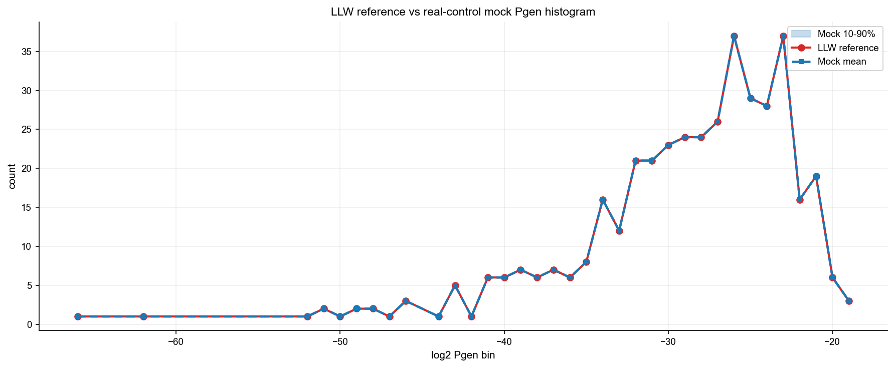
Why real control?#
Using a real human TRB control repertoire instead of a fully synthetic OLGA null corrects for biases that OLGA does not model: sequencing depth artifacts, PCR amplification skew, and repertoire sampling effects.
For this section we also compute V/J adjustment against the real control distribution (YF / real-control usage), not YF / OLGA. OLGA-based adjustment is kept for the synthetic-null comparison in section 9.
The histogram above should show that the real-control mock bin distribution (blue dashes) is close to the LLW reference (red). A large discrepancy would indicate that Pgen or gene-usage adjustment requires further tuning.
After the mock key sets are built here (lazy, first .score() call), each subsequent .score() call reuses them — only the query-repertoire counting differs per sample.
[6]:
real_result = build_real_control_analysis(
    vdjdb_rep,
    yfv_gu,
    seed=SEED,
    count_mode=USAGE_COUNT_MODE,
    pseudocount=USAGE_PSEUDOCOUNT,
    pool_size=POOL_SIZE,
    n_mocks=N_MOCKS,
    n_jobs=8,
)

real_control_df = real_result.control_df
real_control_gu = real_result.control_usage
pgen_adj_real = real_result.pgen_adj_real
pool = real_result.pool
analysis = real_result.analysis
dt = real_result.elapsed_s
print(f"Pool built: n_generated={pool.n_generated:,}, bins={len(pool.bins)}, floor={pool.floor_bin}, ceil={pool.ceil_bin}, elapsed={dt:.1f}s")

diag = compute_bin_alignment_diagnostics(analysis)
all_bins = diag["all_bins"]
ref_vec = diag["ref_vec"]
mock_mat = diag["mock_mat"]
mock_mean = diag["mock_mean"]
mock_q10 = diag["mock_q10"]
mock_q90 = diag["mock_q90"]
max_abs_diff = diag["max_abs_diff"]
rmsd = diag["rmsd"]

fig, ax = plt.subplots(figsize=(12, 5))
ax.fill_between(all_bins, mock_q10, mock_q90, alpha=0.25, color="#1f77b4", label="Mock 10-90%", zorder=1)
ax.plot(all_bins, ref_vec, color="#d62728", marker="o", linewidth=2, label="LLW reference", zorder=2)
# Draw mock mean last so it remains visible even when overlapping the reference line.
ax.plot(all_bins, mock_mean, color="#1f77b4", linestyle="--", marker="s", markersize=4, linewidth=2.2, label="Mock mean", zorder=3)
ax.set_xlabel("log2 Pgen bin")
ax.set_ylabel("count")
ax.set_title("LLW reference vs real-control mock Pgen histogram")
ax.legend()
ax.grid(alpha=0.2)
plt.tight_layout()
plt.show()

print(f"Mock vs LLW: median max|Delta p(bin)|={np.median(max_abs_diff):.4f}, p95={np.percentile(max_abs_diff,95):.4f}")
print(f"Mock vs LLW: median RMSD={np.median(rmsd):.4f}, p95={np.percentile(rmsd,95):.4f}")
Pool built: n_generated=99,981, bins=49, floor=-66, ceil=-18, elapsed=96.8s
Mock vs LLW: median max|Delta p(bin)|=0.0000, p95=0.0000
Mock vs LLW: median RMSD=0.0000, p95=0.0000
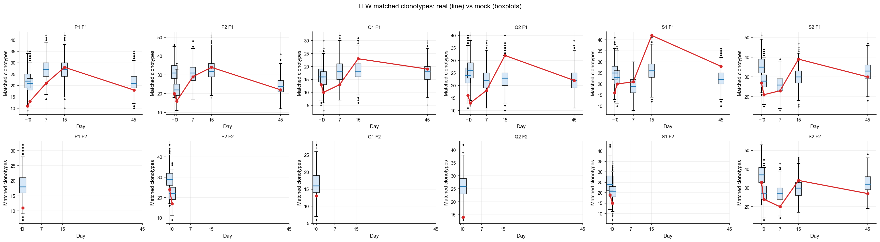
5. LLW overlap per sample: matched clonotypes and duplicate_count#
Compute for each donor/day/replica:
real LLW overlap
mock distribution summary
z-score and empirical p-value
Cohen d
FDR-adjusted p-values
[7]:
df_res = score_samples_dataframe(analysis, samples, progress_every=10, sample_n_jobs=8)
# Convert Polars → pandas; downstream cells use pandas API (iterrows, pivot_table, etc.)
if hasattr(df_res, "to_pandas"):
    df_res = df_res.to_pandas()

display(df_res[[
    "donor", "replica", "day",
    "matched_n_real", "matched_dc_real", "matched_n_fraction", "matched_dc_fraction",
    "matched_n_mock_mean", "matched_n_z", "matched_n_p_emp", "matched_n_cohen_d",
    "matched_dc_log2_real", "matched_dc_log2_mock_mean", "matched_dc_log2_z", "matched_dc_log2_p_emp", "matched_dc_log2_cohen_d",
]])
Processed 10/42 samples
Processed 20/42 samples
Processed 30/42 samples
Processed 40/42 samples
| donor | replica | day | matched_n_real | matched_dc_real | matched_n_fraction | matched_dc_fraction | matched_n_mock_mean | matched_n_z | matched_n_p_emp | matched_n_cohen_d | matched_dc_log2_real | matched_dc_log2_mock_mean | matched_dc_log2_z | matched_dc_log2_p_emp | matched_dc_log2_cohen_d | |
|---|---|---|---|---|---|---|---|---|---|---|---|---|---|---|---|---|
| 0 | P1 | F1 | -1 | 11.0 | 55.0 | 0.000017 | 0.000049 | 21.733 | -2.528267 | 0.999001 | -2.528267 | 5.807355 | 5.852050 | -0.089607 | 0.525475 | -0.089607 |
| 1 | P1 | F1 | 0 | 13.0 | 48.0 | 0.000022 | 0.000057 | 20.682 | -1.913755 | 0.991009 | -1.913755 | 5.614710 | 5.436454 | 0.391387 | 0.355644 | 0.391387 |
| 2 | P1 | F1 | 7 | 21.0 | 100.0 | 0.000025 | 0.000062 | 27.058 | -1.306924 | 0.931069 | -1.306924 | 6.658211 | 6.369355 | 0.581491 | 0.265734 | 0.581491 |
| 3 | P1 | F1 | 15 | 28.0 | 364.0 | 0.000031 | 0.000206 | 27.009 | 0.216564 | 0.444555 | 0.216564 | 8.511753 | 6.457772 | 3.232702 | 0.020979 | 3.232702 |
| 4 | P1 | F1 | 45 | 18.0 | 432.0 | 0.000030 | 0.000452 | 21.247 | -0.767548 | 0.820180 | -0.767548 | 8.758223 | 5.732641 | 5.786307 | 0.000999 | 5.786307 |
| 5 | P1 | F2 | 0 | 11.0 | 45.0 | 0.000021 | 0.000058 | 18.572 | -1.881685 | 0.984016 | -1.881685 | 5.523562 | 5.249873 | 0.548540 | 0.305694 | 0.548540 |
| 6 | P2 | F1 | -1 | 20.0 | 61.0 | 0.000019 | 0.000028 | 31.375 | -2.276396 | 0.995005 | -2.276396 | 5.954196 | 6.817136 | -1.359797 | 0.971029 | -1.359797 |
| 7 | P2 | F1 | 0 | 16.0 | 41.0 | 0.000026 | 0.000042 | 21.875 | -1.380711 | 0.945055 | -1.380711 | 5.392317 | 5.736150 | -0.618093 | 0.781219 | -0.618093 |
| 8 | P2 | F1 | 7 | 29.0 | 88.0 | 0.000026 | 0.000038 | 30.789 | -0.363601 | 0.673327 | -0.363601 | 6.475733 | 6.795364 | -0.496604 | 0.714286 | -0.496604 |
| 9 | P2 | F1 | 15 | 34.0 | 278.0 | 0.000029 | 0.000128 | 32.486 | 0.296556 | 0.422577 | 0.296556 | 8.124121 | 6.744152 | 2.392145 | 0.025974 | 2.392145 |
| 10 | P2 | F1 | 45 | 22.0 | 95.0 | 0.000030 | 0.000074 | 24.309 | -0.526232 | 0.734266 | -0.526232 | 6.584963 | 6.083955 | 0.844796 | 0.125874 | 0.844796 |
| 11 | P2 | F2 | -1 | 24.0 | 65.0 | 0.000025 | 0.000034 | 29.036 | -1.046087 | 0.884116 | -1.046087 | 6.044394 | 6.637700 | -0.914796 | 0.881119 | -0.914796 |
| 12 | P2 | F2 | 0 | 17.0 | 25.0 | 0.000027 | 0.000025 | 21.797 | -1.133511 | 0.895105 | -1.133511 | 4.700440 | 5.727567 | -1.863944 | 0.993007 | -1.863944 |
| 13 | Q1 | F1 | -1 | 13.0 | 101.0 | 0.000033 | 0.000109 | 16.173 | -0.863563 | 0.839161 | -0.863563 | 6.672425 | 5.294234 | 1.811331 | 0.059940 | 1.811331 |
| 14 | Q1 | F1 | 0 | 10.0 | 58.0 | 0.000027 | 0.000072 | 15.908 | -1.602554 | 0.972028 | -1.602554 | 5.882643 | 4.994632 | 1.359688 | 0.090909 | 1.359688 |
| 15 | Q1 | F1 | 7 | 13.0 | 97.0 | 0.000029 | 0.000093 | 17.935 | -1.259349 | 0.927073 | -1.259349 | 6.614710 | 5.444051 | 1.619213 | 0.070929 | 1.619213 |
| 16 | Q1 | F1 | 15 | 23.0 | 237.0 | 0.000051 | 0.000281 | 18.464 | 1.144622 | 0.148851 | 1.144622 | 7.894818 | 5.328034 | 4.164496 | 0.000999 | 4.164496 |
| 17 | Q1 | F1 | 45 | 19.0 | 85.0 | 0.000043 | 0.000102 | 17.543 | 0.397169 | 0.393606 | 0.397169 | 6.426265 | 5.340650 | 1.636933 | 0.076923 | 1.636933 |
| 18 | Q1 | F2 | 0 | 13.0 | 60.0 | 0.000033 | 0.000065 | 16.339 | -0.938175 | 0.857143 | -0.938175 | 5.930737 | 5.106298 | 1.296140 | 0.098901 | 1.296140 |
| 19 | Q2 | F1 | -1 | 16.0 | 43.0 | 0.000025 | 0.000028 | 24.353 | -1.840431 | 0.985015 | -1.840431 | 5.459432 | 6.213564 | -1.023026 | 0.917083 | -1.023026 |
| 20 | Q2 | F1 | 0 | 13.0 | 32.0 | 0.000019 | 0.000023 | 25.906 | -2.846177 | 0.999001 | -2.846177 | 5.044394 | 6.189693 | -1.561570 | 0.986014 | -1.561570 |
| 21 | Q2 | F1 | 7 | 18.0 | 35.0 | 0.000030 | 0.000020 | 22.224 | -0.995003 | 0.863137 | -0.995003 | 5.169925 | 6.432626 | -1.424500 | 0.980020 | -1.424500 |
| 22 | Q2 | F1 | 15 | 32.0 | 214.0 | 0.000053 | 0.000148 | 23.039 | 2.115927 | 0.030969 | 2.115927 | 7.748193 | 6.200783 | 2.005965 | 0.034965 | 2.005965 |
| 23 | Q2 | F1 | 45 | 22.0 | 48.0 | 0.000039 | 0.000033 | 22.172 | -0.039240 | 0.547453 | -0.039240 | 5.614710 | 6.157814 | -0.565967 | 0.770230 | -0.565967 |
| 24 | Q2 | F2 | 0 | 14.0 | 24.0 | 0.000020 | 0.000016 | 25.848 | -2.562470 | 0.999001 | -2.562470 | 4.643856 | 6.307501 | -2.289550 | 1.000000 | -2.289550 |
| 25 | S1 | F1 | -1 | 16.0 | 47.0 | 0.000024 | 0.000042 | 25.112 | -2.064365 | 0.988012 | -2.064365 | 5.584963 | 6.137874 | -0.956872 | 0.849151 | -0.956872 |
| 26 | S1 | F1 | 0 | 20.0 | 66.0 | 0.000037 | 0.000071 | 22.855 | -0.647971 | 0.772228 | -0.647971 | 6.066089 | 5.916064 | 0.252305 | 0.357642 | 0.252305 |
| 27 | S1 | F1 | 7 | 21.0 | 32.0 | 0.000049 | 0.000049 | 19.118 | 0.476927 | 0.347652 | 0.476927 | 5.044394 | 5.401170 | -0.611822 | 0.773227 | -0.611822 |
| 28 | S1 | F1 | 15 | 42.0 | 814.0 | 0.000063 | 0.000761 | 25.978 | 3.463383 | 0.000999 | 3.463383 | 9.670656 | 6.058359 | 6.332003 | 0.000999 | 6.332003 |
| 29 | S1 | F1 | 45 | 28.0 | 368.0 | 0.000049 | 0.000378 | 22.422 | 1.370948 | 0.109890 | 1.370948 | 8.527477 | 5.825460 | 4.589465 | 0.003996 | 4.589465 |
| 30 | S1 | F2 | -1 | 19.0 | 51.0 | 0.000030 | 0.000048 | 24.513 | -1.238716 | 0.910090 | -1.238716 | 5.700440 | 6.058294 | -0.610654 | 0.753247 | -0.610654 |
| 31 | S1 | F2 | 0 | 15.0 | 35.0 | 0.000032 | 0.000045 | 20.663 | -1.341158 | 0.937063 | -1.341158 | 5.169925 | 5.654028 | -0.787073 | 0.816184 | -0.787073 |
| 32 | S2 | F1 | -1 | 27.0 | 77.0 | 0.000026 | 0.000036 | 35.406 | -1.603117 | 0.958042 | -1.603117 | 6.285402 | 7.130760 | -1.703762 | 0.979021 | -1.703762 |
| 33 | S2 | F1 | 0 | 21.0 | 54.0 | 0.000030 | 0.000040 | 27.917 | -1.454915 | 0.953047 | -1.454915 | 5.781360 | 6.427097 | -1.334847 | 0.929071 | -1.334847 |
| 34 | S2 | F1 | 7 | 23.0 | 73.0 | 0.000034 | 0.000050 | 25.855 | -0.606896 | 0.755245 | -0.606896 | 6.209453 | 6.482263 | -0.503692 | 0.710290 | -0.503692 |
| 35 | S2 | F1 | 15 | 39.0 | 471.0 | 0.000048 | 0.000292 | 30.088 | 1.865387 | 0.046953 | 1.865387 | 8.882643 | 6.664434 | 4.116877 | 0.005994 | 4.116877 |
| 36 | S2 | F1 | 45 | 30.0 | 67.0 | 0.000032 | 0.000039 | 32.719 | -0.548777 | 0.726274 | -0.548777 | 6.087463 | 6.771117 | -1.319493 | 0.949051 | -1.319493 |
| 37 | S2 | F2 | -1 | 33.0 | 138.0 | 0.000029 | 0.000057 | 37.320 | -0.800567 | 0.799201 | -0.800567 | 7.118941 | 7.277645 | -0.319066 | 0.615385 | -0.319066 |
| 38 | S2 | F2 | 0 | 24.0 | 60.0 | 0.000034 | 0.000046 | 27.409 | -0.700288 | 0.786214 | -0.700288 | 5.930737 | 6.376660 | -0.874301 | 0.837163 | -0.874301 |
| 39 | S2 | F2 | 7 | 20.0 | 71.0 | 0.000028 | 0.000045 | 27.105 | -1.461006 | 0.958042 | -1.461006 | 6.169925 | 6.595491 | -0.799844 | 0.808192 | -0.799844 |
| 40 | S2 | F2 | 15 | 34.0 | 424.0 | 0.000043 | 0.000274 | 29.750 | 0.842204 | 0.218781 | 0.842204 | 8.731319 | 6.590215 | 3.941494 | 0.008991 | 3.941494 |
| 41 | S2 | F2 | 45 | 27.0 | 73.0 | 0.000031 | 0.000045 | 32.283 | -1.063006 | 0.881119 | -1.063006 | 6.209453 | 6.701391 | -0.941058 | 0.867133 | -0.941058 |
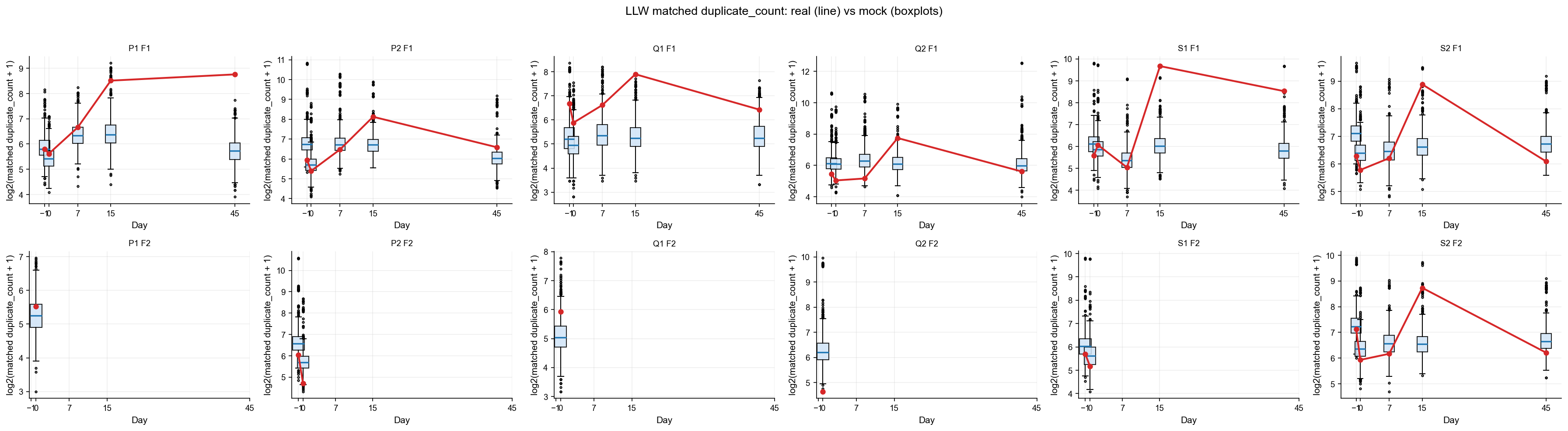
Reading the overlap results#
Four metrics are tracked per sample:
matched_n_real — number of unique LLW CDR3+V+J clonotypes found in the sample.
matched_dc_real — sum of
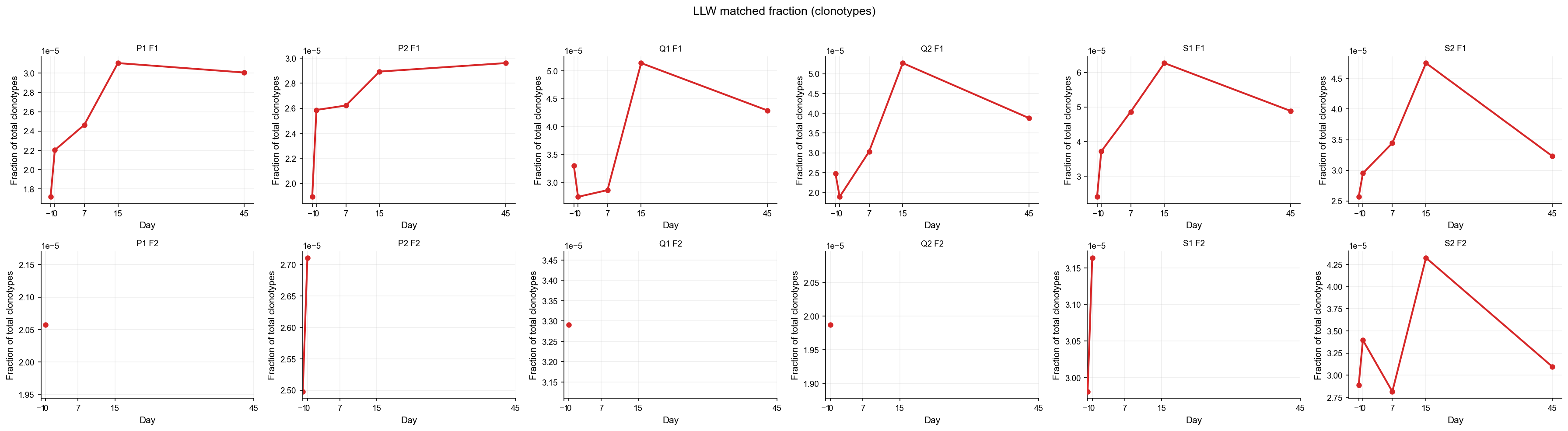
duplicate_countover those matched clonotypes (read depth of the match).matched_n_fraction —
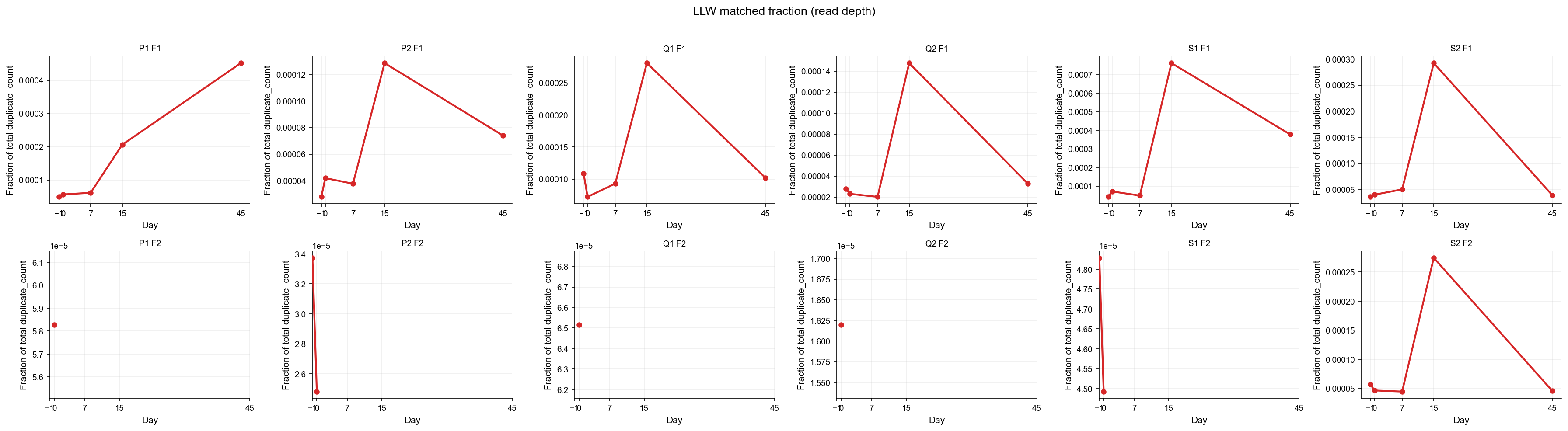
matched_n / n_total(fraction of unique clonotypes in the sample that are LLW).matched_dc_fraction —
matched_dc / dc_total(fraction of total read depth contributed by LLW matches).
Z-scores and Cohen d values are computed relative to the real-control mock null; positive values indicate enrichment above expectation.
[8]:
plot_rows = []
for _, r in df_res.iterrows():
    for x in r["mock_n"]:
        plot_rows.append({
            "donor": r["donor"], "replica": r["replica"], "day": int(r["day"]),
            "metric": "matched_n", "kind": "mock", "value": float(x),
        })
    plot_rows.append({
        "donor": r["donor"], "replica": r["replica"], "day": int(r["day"]),
        "metric": "matched_n", "kind": "real", "value": float(r["matched_n_real"]),
    })
    # Sum of duplicate_count for matched clonotypes (raw read depth of LLW signal)
    for x in r["mock_dc_log2"]:
        plot_rows.append({
            "donor": r["donor"], "replica": r["replica"], "day": int(r["day"]),
            "metric": "matched_dc_log2", "kind": "mock", "value": float(x),
        })
    plot_rows.append({
        "donor": r["donor"], "replica": r["replica"], "day": int(r["day"]),
        "metric": "matched_dc_log2", "kind": "real", "value": float(r["matched_dc_log2_real"]),
    })
    # Fraction of unique clonotypes in sample that are LLW-matched
    plot_rows.append({
        "donor": r["donor"], "replica": r["replica"], "day": int(r["day"]),
        "metric": "matched_n_fraction", "kind": "real", "value": float(r["matched_n_fraction"]),
    })
    # Fraction of total read depth contributed by LLW matches
    plot_rows.append({
        "donor": r["donor"], "replica": r["replica"], "day": int(r["day"]),
        "metric": "matched_dc_fraction", "kind": "real", "value": float(r["matched_dc_fraction"]),
    })

plot_df = pd.DataFrame(plot_rows)
days_all = sorted(df_res["day"].unique().tolist())
donors = sorted(df_res["donor"].unique().tolist())
replicas = sorted(df_res["replica"].unique().tolist())


def draw_panel(metric, ylabel, title, with_mock=True):
    """Draw a grid of per-donor/replica line (real) + optional boxplot (mock) subplots."""
    fig, axes = plt.subplots(
        len(replicas), len(donors),
        figsize=(4.0 * len(donors), 3.2 * len(replicas)),
        squeeze=False,
    )
    fig.suptitle(title, fontsize=13, y=1.02)
    for ri, rep in enumerate(replicas):
        for di, donor in enumerate(donors):
            ax = axes[ri, di]
            sub = plot_df[
                (plot_df["metric"] == metric)
                & (plot_df["donor"] == donor)
                & (plot_df["replica"] == rep)
            ]
            if sub.empty:
                ax.set_visible(False)
                continue

            real = sub[sub["kind"] == "real"].sort_values("day")
            if with_mock:
                mock = sub[sub["kind"] == "mock"]
                box_data = [mock[mock["day"] == d]["value"].values for d in days_all]
                width = 2.5
                ax.boxplot(
                    box_data,
                    positions=days_all,
                    widths=width,
                    patch_artist=True,
                    boxprops=dict(facecolor="#d0e4f7", alpha=0.85),
                    medianprops=dict(color="#1f77b4", linewidth=1.6),
                    flierprops=dict(markersize=2),
                    manage_ticks=False,
                )
            ax.plot(real["day"], real["value"], "-o", color="#d62728", linewidth=2, markersize=5, zorder=5)
            ax.set_xticks(days_all)
            ax.set_xlabel("Day")
            ax.set_ylabel(ylabel)
            ax.set_title(f"{donor} {rep}", fontsize=9)
            ax.grid(alpha=0.2)

    plt.tight_layout()
    plt.show()


draw_panel("matched_n", "Matched clonotypes", "LLW matched clonotypes: real (line) vs mock (boxplots)")
draw_panel("matched_dc_log2", "log2(matched duplicate_count + 1)", "LLW matched duplicate_count: real (line) vs mock (boxplots)")
draw_panel("matched_n_fraction", "Fraction of total clonotypes", "LLW matched fraction (clonotypes)", with_mock=False)
draw_panel("matched_dc_fraction", "Fraction of total duplicate_count", "LLW matched fraction (read depth)", with_mock=False)
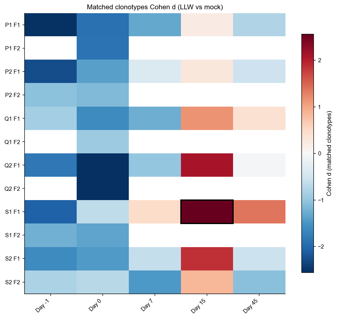
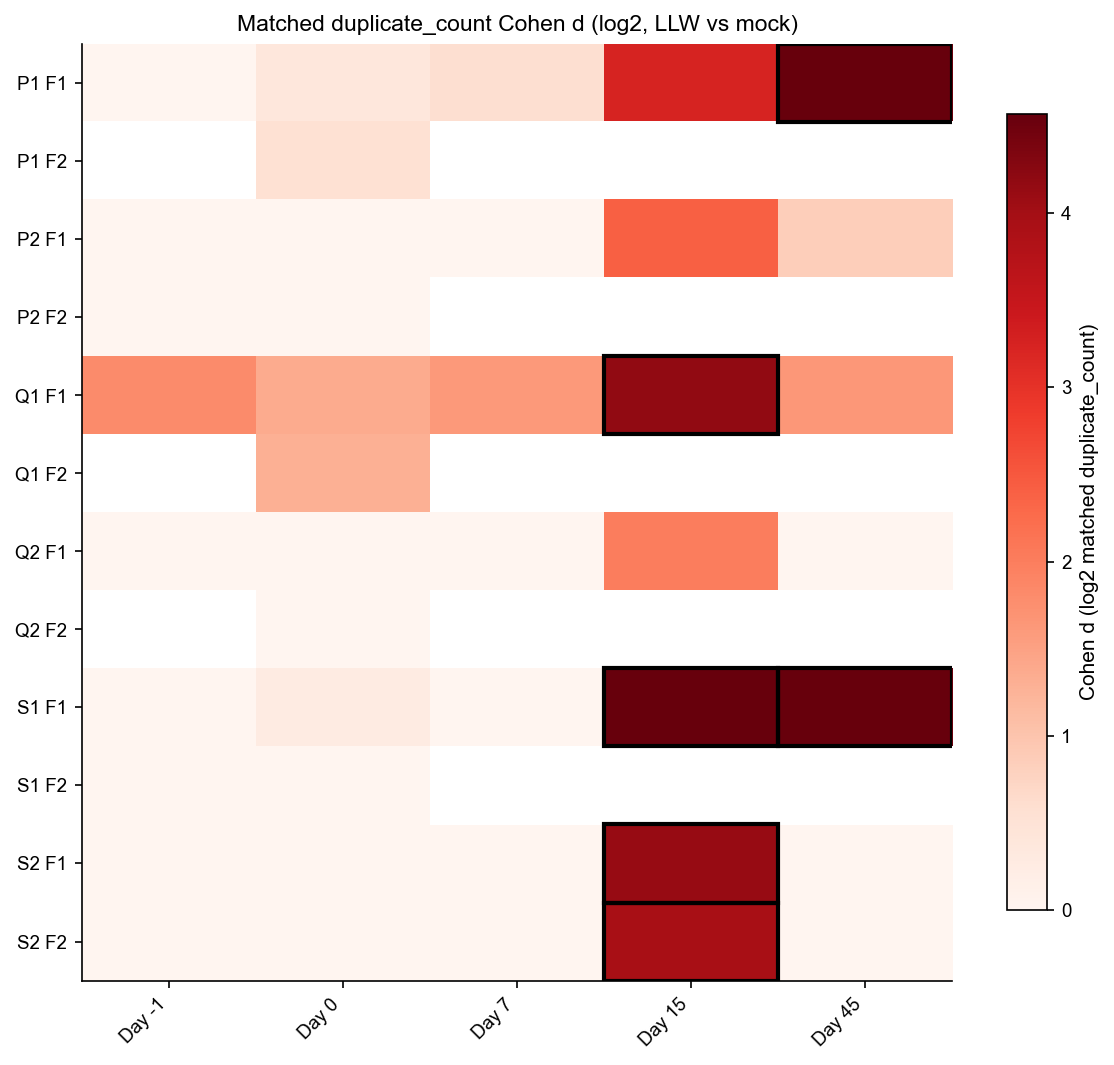
7. Cohen d heatmaps#
[9]:
def heatmap_cohen(value_col, p_adj_col, title, cbar_label, cmap="RdBu_r", vlim=None):
    work = df_res.copy()
    work["sample"] = work["donor"] + " " + work["replica"]
    pv = work.pivot_table(index="sample", columns="day", values=value_col, aggfunc="first")
    pp = work.pivot_table(index="sample", columns="day", values=p_adj_col, aggfunc="first")

    mat = pv.values.astype(float)
    if vlim is None:
        vmax = max(1.0, np.nanpercentile(np.abs(mat), 95))
        vmin = -vmax
    else:
        vmin, vmax = vlim

    fig, ax = plt.subplots(figsize=(8, max(3.5, 0.6 * pv.shape[0])))
    im = ax.imshow(mat, cmap=cmap, aspect="auto", vmin=vmin, vmax=vmax, interpolation="nearest")
    cb = plt.colorbar(im, ax=ax, shrink=0.85)
    cb.set_label(cbar_label)

    for r in range(pv.shape[0]):
        for c in range(pv.shape[1]):
            p = pp.values[r, c]
            d = pv.values[r, c]
            if pd.notna(p) and pd.notna(d) and (float(p) < 0.10) and (float(d) > 0):
                ax.add_patch(plt.Rectangle((c - 0.5, r - 0.5), 1, 1, fill=False, edgecolor="black", linewidth=2))

    ax.set_xticks(range(len(pv.columns)))
    ax.set_xticklabels([f"Day {d}" for d in pv.columns], rotation=45, ha="right")
    ax.set_yticks(range(len(pv.index)))
    ax.set_yticklabels(pv.index)
    ax.set_title(title)
    plt.tight_layout()
    plt.show()

heatmap_cohen(
    value_col="matched_n_cohen_d",
    p_adj_col="matched_n_p_adj",
    title="Matched clonotypes Cohen d (LLW vs mock)",
    cbar_label="Cohen d (matched clonotypes)",
    cmap="RdBu_r",
)

heatmap_cohen(
    value_col="matched_dc_log2_cohen_d",
    p_adj_col="matched_dc_log2_p_adj",
    title="Matched duplicate_count Cohen d (log2, LLW vs mock)",
    cbar_label="Cohen d (log2 matched duplicate_count)",
    cmap="Reds",
    vlim=(0, max(1.0, np.nanpercentile(df_res["matched_dc_log2_cohen_d"].values, 95))),
)
8. Final summary tables#
[10]:
summary_cols = [
    "donor", "replica", "day",
    "n_total", "dc_total",
    "matched_n_real", "matched_dc_real", "matched_n_fraction", "matched_dc_fraction",
    "matched_n_mock_mean", "matched_n_mock_sd", "matched_n_cohen_d", "matched_n_z", "matched_n_p_emp", "matched_n_p_adj",
    "matched_dc_log2_real", "matched_dc_log2_mock_mean", "matched_dc_log2_mock_sd",
    "matched_dc_log2_cohen_d", "matched_dc_log2_z", "matched_dc_log2_p_emp", "matched_dc_log2_p_adj",
]
summary = df_res[summary_cols].copy()
for col in [
    "matched_n_real", "matched_dc_real",
    "matched_n_mock_mean", "matched_n_mock_sd", "matched_n_cohen_d", "matched_n_z",
    "matched_dc_log2_real", "matched_dc_log2_mock_mean", "matched_dc_log2_mock_sd", "matched_dc_log2_cohen_d", "matched_dc_log2_z",
]:
    summary[col] = summary[col].astype(float).round(3)
for col in ["matched_n_fraction", "matched_dc_fraction"]:
    summary[col] = summary[col].map(lambda x: f"{x:.5f}")
for col in ["matched_n_p_emp", "matched_n_p_adj", "matched_dc_log2_p_emp", "matched_dc_log2_p_adj"]:
    summary[col] = summary[col].map(lambda x: f"{x:.4f}")

display(summary.sort_values(["donor", "replica", "day"]).reset_index(drop=True))

print("Top positive matched clonotype effects by Cohen d:")
display(summary.sort_values("matched_n_cohen_d", ascending=False).head(12))

print("Top positive matched duplicate_count effects by Cohen d:")
display(summary.sort_values("matched_dc_log2_cohen_d", ascending=False).head(12))
| donor | replica | day | n_total | dc_total | matched_n_real | matched_dc_real | matched_n_fraction | matched_dc_fraction | matched_n_mock_mean | ... | matched_n_z | matched_n_p_emp | matched_n_p_adj | matched_dc_log2_real | matched_dc_log2_mock_mean | matched_dc_log2_mock_sd | matched_dc_log2_cohen_d | matched_dc_log2_z | matched_dc_log2_p_emp | matched_dc_log2_p_adj | |
|---|---|---|---|---|---|---|---|---|---|---|---|---|---|---|---|---|---|---|---|---|---|
| 0 | P1 | F1 | -1 | 640262 | 1113509 | 11.0 | 55.0 | 0.00002 | 0.00005 | 21.733 | ... | -2.528 | 0.9990 | 0.9990 | 5.807 | 5.852 | 0.499 | -0.090 | -0.090 | 0.5255 | 1.0000 |
| 1 | P1 | F1 | 0 | 590253 | 848323 | 13.0 | 48.0 | 0.00002 | 0.00006 | 20.682 | ... | -1.914 | 0.9910 | 0.9990 | 5.615 | 5.436 | 0.455 | 0.391 | 0.391 | 0.3556 | 0.7906 |
| 2 | P1 | F1 | 7 | 852394 | 1623860 | 21.0 | 100.0 | 0.00002 | 0.00006 | 27.058 | ... | -1.307 | 0.9311 | 0.9990 | 6.658 | 6.369 | 0.497 | 0.581 | 0.581 | 0.2657 | 0.6976 |
| 3 | P1 | F1 | 15 | 901914 | 1764263 | 28.0 | 364.0 | 0.00003 | 0.00021 | 27.009 | ... | 0.217 | 0.4446 | 0.9990 | 8.512 | 6.458 | 0.635 | 3.233 | 3.233 | 0.0210 | 0.1259 |
| 4 | P1 | F1 | 45 | 598677 | 956614 | 18.0 | 432.0 | 0.00003 | 0.00045 | 21.247 | ... | -0.768 | 0.8202 | 0.9990 | 8.758 | 5.733 | 0.523 | 5.786 | 5.786 | 0.0010 | 0.0140 |
| 5 | P1 | F2 | 0 | 534632 | 772165 | 11.0 | 45.0 | 0.00002 | 0.00006 | 18.572 | ... | -1.882 | 0.9840 | 0.9990 | 5.524 | 5.250 | 0.499 | 0.549 | 0.549 | 0.3057 | 0.7552 |
| 6 | P2 | F1 | -1 | 1056617 | 2177498 | 20.0 | 61.0 | 0.00002 | 0.00003 | 31.375 | ... | -2.276 | 0.9950 | 0.9990 | 5.954 | 6.817 | 0.635 | -1.360 | -1.360 | 0.9710 | 1.0000 |
| 7 | P2 | F1 | 0 | 618627 | 974518 | 16.0 | 41.0 | 0.00003 | 0.00004 | 21.875 | ... | -1.381 | 0.9451 | 0.9990 | 5.392 | 5.736 | 0.556 | -0.618 | -0.618 | 0.7812 | 1.0000 |
| 8 | P2 | F1 | 7 | 1106211 | 2324263 | 29.0 | 88.0 | 0.00003 | 0.00004 | 30.789 | ... | -0.364 | 0.6733 | 0.9990 | 6.476 | 6.795 | 0.644 | -0.497 | -0.497 | 0.7143 | 1.0000 |
| 9 | P2 | F1 | 15 | 1175459 | 2165475 | 34.0 | 278.0 | 0.00003 | 0.00013 | 32.486 | ... | 0.297 | 0.4226 | 0.9990 | 8.124 | 6.744 | 0.577 | 2.392 | 2.392 | 0.0260 | 0.1364 |
| 10 | P2 | F1 | 45 | 743145 | 1284712 | 22.0 | 95.0 | 0.00003 | 0.00007 | 24.309 | ... | -0.526 | 0.7343 | 0.9990 | 6.585 | 6.084 | 0.593 | 0.845 | 0.845 | 0.1259 | 0.3524 |
| 11 | P2 | F2 | -1 | 960830 | 1926603 | 24.0 | 65.0 | 0.00002 | 0.00003 | 29.036 | ... | -1.046 | 0.8841 | 0.9990 | 6.044 | 6.638 | 0.649 | -0.915 | -0.915 | 0.8811 | 1.0000 |
| 12 | P2 | F2 | 0 | 627140 | 1007567 | 17.0 | 25.0 | 0.00003 | 0.00002 | 21.797 | ... | -1.134 | 0.8951 | 0.9990 | 4.700 | 5.728 | 0.551 | -1.864 | -1.864 | 0.9930 | 1.0000 |
| 13 | Q1 | F1 | -1 | 393851 | 930778 | 13.0 | 101.0 | 0.00003 | 0.00011 | 16.173 | ... | -0.864 | 0.8392 | 0.9990 | 6.672 | 5.294 | 0.761 | 1.811 | 1.811 | 0.0599 | 0.2517 |
| 14 | Q1 | F1 | 0 | 365046 | 801690 | 10.0 | 58.0 | 0.00003 | 0.00007 | 15.908 | ... | -1.603 | 0.9720 | 0.9990 | 5.883 | 4.995 | 0.653 | 1.360 | 1.360 | 0.0909 | 0.2937 |
| 15 | Q1 | F1 | 7 | 454574 | 1042775 | 13.0 | 97.0 | 0.00003 | 0.00009 | 17.935 | ... | -1.259 | 0.9271 | 0.9990 | 6.615 | 5.444 | 0.723 | 1.619 | 1.619 | 0.0709 | 0.2692 |
| 16 | Q1 | F1 | 15 | 447584 | 843549 | 23.0 | 237.0 | 0.00005 | 0.00028 | 18.464 | ... | 1.145 | 0.1489 | 0.9990 | 7.895 | 5.328 | 0.616 | 4.164 | 4.164 | 0.0010 | 0.0140 |
| 17 | Q1 | F1 | 45 | 442934 | 833618 | 19.0 | 85.0 | 0.00004 | 0.00010 | 17.543 | ... | 0.397 | 0.3936 | 0.9990 | 6.426 | 5.341 | 0.663 | 1.637 | 1.637 | 0.0769 | 0.2692 |
| 18 | Q1 | F2 | 0 | 395028 | 920754 | 13.0 | 60.0 | 0.00003 | 0.00007 | 16.339 | ... | -0.938 | 0.8571 | 0.9990 | 5.931 | 5.106 | 0.636 | 1.296 | 1.296 | 0.0989 | 0.2967 |
| 19 | Q2 | F1 | -1 | 644960 | 1551950 | 16.0 | 43.0 | 0.00002 | 0.00003 | 24.353 | ... | -1.840 | 0.9850 | 0.9990 | 5.459 | 6.214 | 0.737 | -1.023 | -1.023 | 0.9171 | 1.0000 |
| 20 | Q2 | F1 | 0 | 688166 | 1391788 | 13.0 | 32.0 | 0.00002 | 0.00002 | 25.906 | ... | -2.846 | 0.9990 | 0.9990 | 5.044 | 6.190 | 0.733 | -1.562 | -1.562 | 0.9860 | 1.0000 |
| 21 | Q2 | F1 | 7 | 593659 | 1736828 | 18.0 | 35.0 | 0.00003 | 0.00002 | 22.224 | ... | -0.995 | 0.8631 | 0.9990 | 5.170 | 6.433 | 0.886 | -1.424 | -1.424 | 0.9800 | 1.0000 |
| 22 | Q2 | F1 | 15 | 607413 | 1449423 | 32.0 | 214.0 | 0.00005 | 0.00015 | 23.039 | ... | 2.116 | 0.0310 | 0.6503 | 7.748 | 6.201 | 0.771 | 2.006 | 2.006 | 0.0350 | 0.1632 |
| 23 | Q2 | F1 | 45 | 567178 | 1464089 | 22.0 | 48.0 | 0.00004 | 0.00003 | 22.172 | ... | -0.039 | 0.5475 | 0.9990 | 5.615 | 6.158 | 0.960 | -0.566 | -0.566 | 0.7702 | 1.0000 |
| 24 | Q2 | F2 | 0 | 704492 | 1481580 | 14.0 | 24.0 | 0.00002 | 0.00002 | 25.848 | ... | -2.562 | 0.9990 | 0.9990 | 4.644 | 6.308 | 0.727 | -2.290 | -2.290 | 1.0000 | 1.0000 |
| 25 | S1 | F1 | -1 | 665282 | 1110908 | 16.0 | 47.0 | 0.00002 | 0.00004 | 25.112 | ... | -2.064 | 0.9880 | 0.9990 | 5.585 | 6.138 | 0.578 | -0.957 | -0.957 | 0.8492 | 1.0000 |
| 26 | S1 | F1 | 0 | 537799 | 925833 | 20.0 | 66.0 | 0.00004 | 0.00007 | 22.855 | ... | -0.648 | 0.7722 | 0.9990 | 6.066 | 5.916 | 0.595 | 0.252 | 0.252 | 0.3576 | 0.7906 |
| 27 | S1 | F1 | 7 | 431736 | 652745 | 21.0 | 32.0 | 0.00005 | 0.00005 | 19.118 | ... | 0.477 | 0.3477 | 0.9990 | 5.044 | 5.401 | 0.583 | -0.612 | -0.612 | 0.7732 | 1.0000 |
| 28 | S1 | F1 | 15 | 669972 | 1069012 | 42.0 | 814.0 | 0.00006 | 0.00076 | 25.978 | ... | 3.463 | 0.0010 | 0.0420 | 9.671 | 6.058 | 0.570 | 6.332 | 6.332 | 0.0010 | 0.0140 |
| 29 | S1 | F1 | 45 | 572955 | 972623 | 28.0 | 368.0 | 0.00005 | 0.00038 | 22.422 | ... | 1.371 | 0.1099 | 0.9990 | 8.527 | 5.825 | 0.589 | 4.589 | 4.589 | 0.0040 | 0.0420 |
| 30 | S1 | F2 | -1 | 637371 | 1056200 | 19.0 | 51.0 | 0.00003 | 0.00005 | 24.513 | ... | -1.239 | 0.9101 | 0.9990 | 5.700 | 6.058 | 0.586 | -0.611 | -0.611 | 0.7532 | 1.0000 |
| 31 | S1 | F2 | 0 | 474096 | 779081 | 15.0 | 35.0 | 0.00003 | 0.00004 | 20.663 | ... | -1.341 | 0.9371 | 0.9990 | 5.170 | 5.654 | 0.615 | -0.787 | -0.787 | 0.8162 | 1.0000 |
| 32 | S2 | F1 | -1 | 1051499 | 2154393 | 27.0 | 77.0 | 0.00003 | 0.00004 | 35.406 | ... | -1.603 | 0.9580 | 0.9990 | 6.285 | 7.131 | 0.496 | -1.704 | -1.704 | 0.9790 | 1.0000 |
| 33 | S2 | F1 | 0 | 711398 | 1356139 | 21.0 | 54.0 | 0.00003 | 0.00004 | 27.917 | ... | -1.455 | 0.9530 | 0.9990 | 5.781 | 6.427 | 0.484 | -1.335 | -1.335 | 0.9291 | 1.0000 |
| 34 | S2 | F1 | 7 | 667613 | 1458612 | 23.0 | 73.0 | 0.00003 | 0.00005 | 25.855 | ... | -0.607 | 0.7552 | 0.9990 | 6.209 | 6.482 | 0.542 | -0.504 | -0.504 | 0.7103 | 1.0000 |
| 35 | S2 | F1 | 15 | 821039 | 1611965 | 39.0 | 471.0 | 0.00005 | 0.00029 | 30.088 | ... | 1.865 | 0.0470 | 0.6573 | 8.883 | 6.664 | 0.539 | 4.117 | 4.117 | 0.0060 | 0.0503 |
| 36 | S2 | F1 | 45 | 927910 | 1731250 | 30.0 | 67.0 | 0.00003 | 0.00004 | 32.719 | ... | -0.549 | 0.7263 | 0.9990 | 6.087 | 6.771 | 0.518 | -1.319 | -1.319 | 0.9491 | 1.0000 |
| 37 | S2 | F2 | -1 | 1142739 | 2426409 | 33.0 | 138.0 | 0.00003 | 0.00006 | 37.320 | ... | -0.801 | 0.7992 | 0.9990 | 7.119 | 7.278 | 0.497 | -0.319 | -0.319 | 0.6154 | 1.0000 |
| 38 | S2 | F2 | 0 | 706729 | 1293819 | 24.0 | 60.0 | 0.00003 | 0.00005 | 27.409 | ... | -0.700 | 0.7862 | 0.9990 | 5.931 | 6.377 | 0.510 | -0.874 | -0.874 | 0.8372 | 1.0000 |
| 39 | S2 | F2 | 7 | 710413 | 1595370 | 20.0 | 71.0 | 0.00003 | 0.00004 | 27.105 | ... | -1.461 | 0.9580 | 0.9990 | 6.170 | 6.595 | 0.532 | -0.800 | -0.800 | 0.8082 | 1.0000 |
| 40 | S2 | F2 | 15 | 786155 | 1544994 | 34.0 | 424.0 | 0.00004 | 0.00027 | 29.750 | ... | 0.842 | 0.2188 | 0.9990 | 8.731 | 6.590 | 0.543 | 3.941 | 3.941 | 0.0090 | 0.0629 |
| 41 | S2 | F2 | 45 | 871599 | 1604659 | 27.0 | 73.0 | 0.00003 | 0.00005 | 32.283 | ... | -1.063 | 0.8811 | 0.9990 | 6.209 | 6.701 | 0.523 | -0.941 | -0.941 | 0.8671 | 1.0000 |
42 rows × 22 columns
Top positive matched clonotype effects by Cohen d:
| donor | replica | day | n_total | dc_total | matched_n_real | matched_dc_real | matched_n_fraction | matched_dc_fraction | matched_n_mock_mean | ... | matched_n_z | matched_n_p_emp | matched_n_p_adj | matched_dc_log2_real | matched_dc_log2_mock_mean | matched_dc_log2_mock_sd | matched_dc_log2_cohen_d | matched_dc_log2_z | matched_dc_log2_p_emp | matched_dc_log2_p_adj | |
|---|---|---|---|---|---|---|---|---|---|---|---|---|---|---|---|---|---|---|---|---|---|
| 28 | S1 | F1 | 15 | 669972 | 1069012 | 42.0 | 814.0 | 0.00006 | 0.00076 | 25.978 | ... | 3.463 | 0.0010 | 0.0420 | 9.671 | 6.058 | 0.570 | 6.332 | 6.332 | 0.0010 | 0.0140 |
| 22 | Q2 | F1 | 15 | 607413 | 1449423 | 32.0 | 214.0 | 0.00005 | 0.00015 | 23.039 | ... | 2.116 | 0.0310 | 0.6503 | 7.748 | 6.201 | 0.771 | 2.006 | 2.006 | 0.0350 | 0.1632 |
| 35 | S2 | F1 | 15 | 821039 | 1611965 | 39.0 | 471.0 | 0.00005 | 0.00029 | 30.088 | ... | 1.865 | 0.0470 | 0.6573 | 8.883 | 6.664 | 0.539 | 4.117 | 4.117 | 0.0060 | 0.0503 |
| 29 | S1 | F1 | 45 | 572955 | 972623 | 28.0 | 368.0 | 0.00005 | 0.00038 | 22.422 | ... | 1.371 | 0.1099 | 0.9990 | 8.527 | 5.825 | 0.589 | 4.589 | 4.589 | 0.0040 | 0.0420 |
| 16 | Q1 | F1 | 15 | 447584 | 843549 | 23.0 | 237.0 | 0.00005 | 0.00028 | 18.464 | ... | 1.145 | 0.1489 | 0.9990 | 7.895 | 5.328 | 0.616 | 4.164 | 4.164 | 0.0010 | 0.0140 |
| 40 | S2 | F2 | 15 | 786155 | 1544994 | 34.0 | 424.0 | 0.00004 | 0.00027 | 29.750 | ... | 0.842 | 0.2188 | 0.9990 | 8.731 | 6.590 | 0.543 | 3.941 | 3.941 | 0.0090 | 0.0629 |
| 27 | S1 | F1 | 7 | 431736 | 652745 | 21.0 | 32.0 | 0.00005 | 0.00005 | 19.118 | ... | 0.477 | 0.3477 | 0.9990 | 5.044 | 5.401 | 0.583 | -0.612 | -0.612 | 0.7732 | 1.0000 |
| 17 | Q1 | F1 | 45 | 442934 | 833618 | 19.0 | 85.0 | 0.00004 | 0.00010 | 17.543 | ... | 0.397 | 0.3936 | 0.9990 | 6.426 | 5.341 | 0.663 | 1.637 | 1.637 | 0.0769 | 0.2692 |
| 9 | P2 | F1 | 15 | 1175459 | 2165475 | 34.0 | 278.0 | 0.00003 | 0.00013 | 32.486 | ... | 0.297 | 0.4226 | 0.9990 | 8.124 | 6.744 | 0.577 | 2.392 | 2.392 | 0.0260 | 0.1364 |
| 3 | P1 | F1 | 15 | 901914 | 1764263 | 28.0 | 364.0 | 0.00003 | 0.00021 | 27.009 | ... | 0.217 | 0.4446 | 0.9990 | 8.512 | 6.458 | 0.635 | 3.233 | 3.233 | 0.0210 | 0.1259 |
| 23 | Q2 | F1 | 45 | 567178 | 1464089 | 22.0 | 48.0 | 0.00004 | 0.00003 | 22.172 | ... | -0.039 | 0.5475 | 0.9990 | 5.615 | 6.158 | 0.960 | -0.566 | -0.566 | 0.7702 | 1.0000 |
| 8 | P2 | F1 | 7 | 1106211 | 2324263 | 29.0 | 88.0 | 0.00003 | 0.00004 | 30.789 | ... | -0.364 | 0.6733 | 0.9990 | 6.476 | 6.795 | 0.644 | -0.497 | -0.497 | 0.7143 | 1.0000 |
12 rows × 22 columns
Top positive matched duplicate_count effects by Cohen d:
| donor | replica | day | n_total | dc_total | matched_n_real | matched_dc_real | matched_n_fraction | matched_dc_fraction | matched_n_mock_mean | ... | matched_n_z | matched_n_p_emp | matched_n_p_adj | matched_dc_log2_real | matched_dc_log2_mock_mean | matched_dc_log2_mock_sd | matched_dc_log2_cohen_d | matched_dc_log2_z | matched_dc_log2_p_emp | matched_dc_log2_p_adj | |
|---|---|---|---|---|---|---|---|---|---|---|---|---|---|---|---|---|---|---|---|---|---|
| 28 | S1 | F1 | 15 | 669972 | 1069012 | 42.0 | 814.0 | 0.00006 | 0.00076 | 25.978 | ... | 3.463 | 0.0010 | 0.0420 | 9.671 | 6.058 | 0.570 | 6.332 | 6.332 | 0.0010 | 0.0140 |
| 4 | P1 | F1 | 45 | 598677 | 956614 | 18.0 | 432.0 | 0.00003 | 0.00045 | 21.247 | ... | -0.768 | 0.8202 | 0.9990 | 8.758 | 5.733 | 0.523 | 5.786 | 5.786 | 0.0010 | 0.0140 |
| 29 | S1 | F1 | 45 | 572955 | 972623 | 28.0 | 368.0 | 0.00005 | 0.00038 | 22.422 | ... | 1.371 | 0.1099 | 0.9990 | 8.527 | 5.825 | 0.589 | 4.589 | 4.589 | 0.0040 | 0.0420 |
| 16 | Q1 | F1 | 15 | 447584 | 843549 | 23.0 | 237.0 | 0.00005 | 0.00028 | 18.464 | ... | 1.145 | 0.1489 | 0.9990 | 7.895 | 5.328 | 0.616 | 4.164 | 4.164 | 0.0010 | 0.0140 |
| 35 | S2 | F1 | 15 | 821039 | 1611965 | 39.0 | 471.0 | 0.00005 | 0.00029 | 30.088 | ... | 1.865 | 0.0470 | 0.6573 | 8.883 | 6.664 | 0.539 | 4.117 | 4.117 | 0.0060 | 0.0503 |
| 40 | S2 | F2 | 15 | 786155 | 1544994 | 34.0 | 424.0 | 0.00004 | 0.00027 | 29.750 | ... | 0.842 | 0.2188 | 0.9990 | 8.731 | 6.590 | 0.543 | 3.941 | 3.941 | 0.0090 | 0.0629 |
| 3 | P1 | F1 | 15 | 901914 | 1764263 | 28.0 | 364.0 | 0.00003 | 0.00021 | 27.009 | ... | 0.217 | 0.4446 | 0.9990 | 8.512 | 6.458 | 0.635 | 3.233 | 3.233 | 0.0210 | 0.1259 |
| 9 | P2 | F1 | 15 | 1175459 | 2165475 | 34.0 | 278.0 | 0.00003 | 0.00013 | 32.486 | ... | 0.297 | 0.4226 | 0.9990 | 8.124 | 6.744 | 0.577 | 2.392 | 2.392 | 0.0260 | 0.1364 |
| 22 | Q2 | F1 | 15 | 607413 | 1449423 | 32.0 | 214.0 | 0.00005 | 0.00015 | 23.039 | ... | 2.116 | 0.0310 | 0.6503 | 7.748 | 6.201 | 0.771 | 2.006 | 2.006 | 0.0350 | 0.1632 |
| 13 | Q1 | F1 | -1 | 393851 | 930778 | 13.0 | 101.0 | 0.00003 | 0.00011 | 16.173 | ... | -0.864 | 0.8392 | 0.9990 | 6.672 | 5.294 | 0.761 | 1.811 | 1.811 | 0.0599 | 0.2517 |
| 17 | Q1 | F1 | 45 | 442934 | 833618 | 19.0 | 85.0 | 0.00004 | 0.00010 | 17.543 | ... | 0.397 | 0.3936 | 0.9990 | 6.426 | 5.341 | 0.663 | 1.637 | 1.637 | 0.0769 | 0.2692 |
| 15 | Q1 | F1 | 7 | 454574 | 1042775 | 13.0 | 97.0 | 0.00003 | 0.00009 | 17.935 | ... | -1.259 | 0.9271 | 0.9990 | 6.615 | 5.444 | 0.723 | 1.619 | 1.619 | 0.0709 | 0.2692 |
12 rows × 22 columns
Notebook output coverage checklist:
V usage YF vs OLGA and correction factors
LLW reference vs mock Pgen histogram alignment
Matched clonotypes and duplicate_count per sample
Cohen d, z-scores, empirical p-values, FDR
Line + boxplot dynamics and Cohen d heatmaps
[11]:
print("Done: notebook rewritten to Rmd-aligned workflow.")
print(f"Samples: {len(samples)}, mocks: {N_MOCKS}, pool size: {POOL_SIZE:,}")
print("Use the summary table above for export/reporting.")
Done: notebook rewritten to Rmd-aligned workflow.
Samples: 42, mocks: 1000, pool size: 100,000
Use the summary table above for export/reporting.
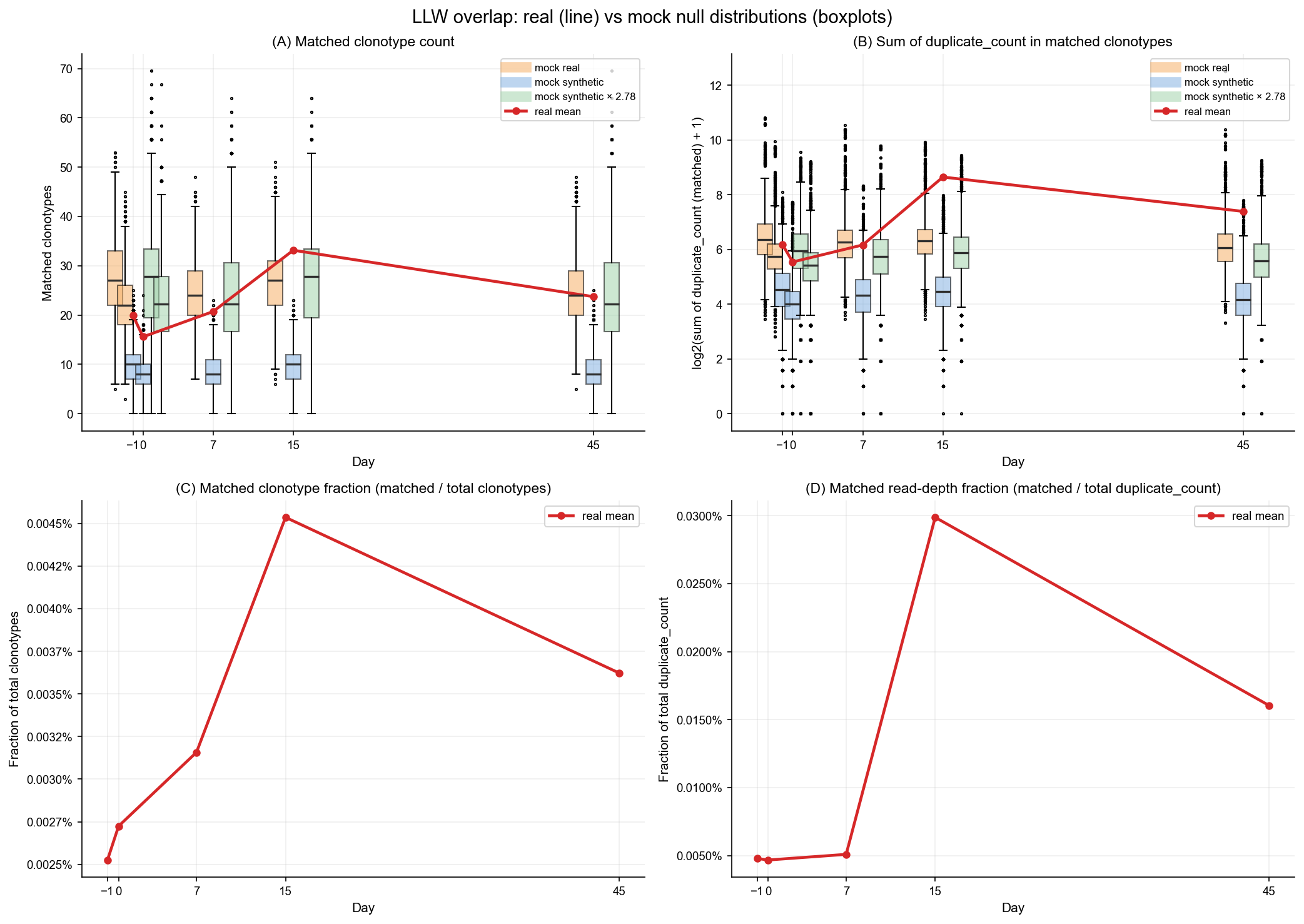
9. Synthetic mock comparison and scale-factor calibration#
Sections 1–8 use a real human TRB control pool to drive the mock null distribution. This section builds a complementary synthetic OLGA pool and rescores all samples under that null, then computes a scale factor \(X\) aligning the two mean mock overlaps:
where \(\bar{m}\) denotes the mean number of mocked matches across all samples. Three mock curves are overlaid per day:
mock real — null from the real-control pool (sections 1–8).
mock synthetic — null from OLGA synthetic sequences.
mock synthetic × X — synthetic rescaled to match the real-pool mean.
The scale factor quantifies how much OLGA under- or over-estimates real-sequence background overlap density. A value \(X > 1\) means the real control finds more background matches than OLGA predicts (typical due to empirical sequence clustering).
[12]:
import importlib
import mir.common.control as _ctrl_mod
import mir.comparative.vdjbet as _vdjbet_mod
importlib.reload(_ctrl_mod)
importlib.reload(_vdjbet_mod)
from mir.comparative.vdjbet import PgenBinPool, VDJBetOverlapAnalysis
print('Reloaded mir.common.control and mir.comparative.vdjbet from source')
Reloaded mir.common.control and mir.comparative.vdjbet from source
[13]:
df_res_real = df_res.copy()  # real-control null from sections 1-8

(
    pool_synth,
    analysis_synth,
    df_res_synth,
    X_scale,
    df_res_synth_scaled,
    ) = build_synthetic_comparison(
        vdjdb_rep,
        samples,
        pgen_adj_olga=pgen_adj_olga,
        pool_size=POOL_SIZE,
        n_mocks=N_MOCKS,
        n_jobs=8,
        seed=SEED,
        sample_n_jobs=8,
        df_res_real=df_res_real,
    )

# Convert Polars → pandas for downstream cells (build_synthetic_comparison returns pl.DataFrame)
if hasattr(df_res_synth, "to_pandas"):
    df_res_synth = df_res_synth.to_pandas()
if hasattr(df_res_synth_scaled, "to_pandas"):
    df_res_synth_scaled = df_res_synth_scaled.to_pandas()

print(f"Synthetic pool records used: {pool_synth.n_generated:,}")
print(f"Synthetic mock mean overlap: {df_res_synth['matched_n_mock_mean'].mean():.4f}")
print(f"Real-control mock mean overlap: {df_res_real['matched_n_mock_mean'].mean():.4f}")
print(f"Scale factor X (real/synthetic): {X_scale:.4f}")
Processed 10/42 samples
Processed 20/42 samples
Processed 30/42 samples
Processed 40/42 samples
Synthetic pool records used: 100,000
Synthetic mock mean overlap: 8.9107
Real-control mock mean overlap: 24.7711
Scale factor X (real/synthetic): 2.7799
[14]:
# Significant hits under real-control null (from sections 1-8).
sig_n_real = df_res_real[
    (df_res_real["matched_n_p_adj"] < 0.10) & (df_res_real["matched_n_cohen_d"] > 0)
]
sig_dc_real = df_res_real[
    (df_res_real["matched_dc_log2_p_adj"] < 0.10) & (df_res_real["matched_dc_log2_cohen_d"] > 0)
]


def _as_triplet_set(df):
    return {(r.donor, r.replica, int(r.day)) for r in df[["donor", "replica", "day"]].itertuples(index=False)}


def _as_label_list(df):
    return [
        f"{r.donor} {r.replica} day {int(r.day)}"
        for r in df[["donor", "replica", "day"]].itertuples(index=False)
    ]


# Expected significant sets based on the YFV19 Rmd analysis (day 15 peak responders).
expected_sig_n = {("S2", "F1", 15), ("S1", "F1", 15), ("Q2", "F1", 15), ("Q1", "F1", 15)}
expected_sig_dc = {
    ("S2", "F1", 15), ("S2", "F2", 15),
    ("S1", "F1", 15), ("S1", "F1", 45),
    ("Q1", "F1", 15),
    ("P2", "F1", 15),
    ("P1", "F1", 15), ("P1", "F1", 45),
}

set_sig_n = _as_triplet_set(sig_n_real)
set_sig_dc = _as_triplet_set(sig_dc_real)

print("Observed significant matched clonotypes (FDR<0.10, d>0):")
print(_as_label_list(sig_n_real))
print("Observed significant matched duplicate_count log2 (FDR<0.10, d>0):")
print(_as_label_list(sig_dc_real))

print("\nExpectation check: matched clonotypes")
print("match:", set_sig_n == expected_sig_n)
print("missing:", sorted(expected_sig_n - set_sig_n))
print("extra:", sorted(set_sig_n - expected_sig_n))

print("\nExpectation check: matched duplicate_count")
print("match:", set_sig_dc == expected_sig_dc)
print("missing:", sorted(expected_sig_dc - set_sig_dc))
print("extra:", sorted(set_sig_dc - expected_sig_dc))

print(f"\nScale factor X (real/synthetic): {X_scale:.3f}")
print("Observation 1: Real-control null captures empirical sequence clustering that OLGA misses.")
print(f"Observation 2: X = {X_scale:.3f} — synthetic mocks undercount overlap by this factor.")
print("Observation 3: Significant calls are exact junction_aa + V + J matching only.")
print("Observation 4: Compare listed observed sets with target day/sample expectations via missing/extra diagnostics.")
Observed significant matched clonotypes (FDR<0.10, d>0):
['S1 F1 day 15']
Observed significant matched duplicate_count log2 (FDR<0.10, d>0):
['P1 F1 day 45', 'Q1 F1 day 15', 'S1 F1 day 15', 'S1 F1 day 45', 'S2 F1 day 15', 'S2 F2 day 15']

Expectation check: matched clonotypes
match: False
missing: [('Q1', 'F1', 15), ('Q2', 'F1', 15), ('S2', 'F1', 15)]
extra: []

Expectation check: matched duplicate_count
match: False
missing: [('P1', 'F1', 15), ('P2', 'F1', 15)]
extra: []

Scale factor X (real/synthetic): 2.780
Observation 1: Real-control null captures empirical sequence clustering that OLGA misses.
Observation 2: X = 2.780 — synthetic mocks undercount overlap by this factor.
Observation 3: Significant calls are exact junction_aa + V + J matching only.
Observation 4: Compare listed observed sets with target day/sample expectations via missing/extra diagnostics.
[15]:
days_plot = sorted(df_res_real["day"].unique().tolist())


def _collect_mock_by_day(df_in, value_col="mock_n", transform=None):
    """Aggregate mock draws per day from a scored DataFrame."""
    out = {d: [] for d in days_plot}
    for _, row in df_in.iterrows():
        d = int(row["day"])
        vals = [float(x) for x in row[value_col]]
        if transform is not None:
            vals = [float(transform(v)) for v in vals]
        out[d].extend(vals)
    return out


real_mock_by_day = _collect_mock_by_day(df_res_real, "mock_n")
syn_mock_by_day = _collect_mock_by_day(df_res_synth, "mock_n")
syn_scaled_mock_by_day = _collect_mock_by_day(df_res_synth_scaled, "mock_n")

# Duplicate-count mock draws are stored as log2(mock_dc + 1). Convert back to raw counts.
_dc_from_log2 = lambda v: (2.0 ** float(v)) - 1.0
real_mock_dc_by_day = _collect_mock_by_day(df_res_real, "mock_dc_log2", transform=_dc_from_log2)
syn_mock_dc_by_day = _collect_mock_by_day(df_res_synth, "mock_dc_log2", transform=_dc_from_log2)
syn_scaled_mock_dc_by_day = _collect_mock_by_day(
    df_res_synth_scaled, "mock_dc_log2", transform=lambda v: _dc_from_log2(v) * X_scale
)

# Real-data mean overlap per day (from sections 1-8, real-control null).
real_mean_by_day = (
    df_res_real.groupby("day", as_index=False)["matched_n_real"].mean().sort_values("day")
)
real_dc_by_day = (
    df_res_real.groupby("day", as_index=False)["matched_dc_real"].mean().sort_values("day")
)
real_frac_n_by_day = (
    df_res_real.groupby("day", as_index=False)["matched_n_fraction"].mean().sort_values("day")
)
real_frac_dc_by_day = (
    df_res_real.groupby("day", as_index=False)["matched_dc_fraction"].mean().sort_values("day")
)

width = 1.5
offsets = [-1.8, 0.0, 1.8]
mock_specs = [
    ("mock real", real_mock_by_day, "#f6b26b", offsets[0]),
    ("mock synthetic", syn_mock_by_day, "#87b4e3", offsets[1]),
    (f"mock synthetic × {X_scale:.2f}", syn_scaled_mock_by_day, "#a4d4ae", offsets[2]),
]
mock_dc_specs = [
    ("mock real", real_mock_dc_by_day, "#f6b26b", offsets[0]),
    ("mock synthetic", syn_mock_dc_by_day, "#87b4e3", offsets[1]),
    (f"mock synthetic × {X_scale:.2f}", syn_scaled_mock_dc_by_day, "#a4d4ae", offsets[2]),
]

fig, axes = plt.subplots(2, 2, figsize=(14, 10))
fig.suptitle("LLW overlap: real (line) vs mock null distributions (boxplots)", fontsize=14)

# ── Panel A: matched clonotype count ──────────────────────────────────────────
ax = axes[0, 0]
for label, by_day, color, off in mock_specs:
    data = [by_day[d] if len(by_day[d]) else [np.nan] for d in days_plot]
    pos = [d + off for d in days_plot]
    ax.boxplot(
        data, positions=pos, widths=width, patch_artist=True, manage_ticks=False,
        boxprops=dict(facecolor=color, alpha=0.55),
        medianprops=dict(color="#2f2f2f", linewidth=1.6),
        flierprops=dict(markersize=1.5),
    )
    ax.plot([], [], color=color, linewidth=8, alpha=0.55, label=label)
ax.plot(real_mean_by_day["day"], real_mean_by_day["matched_n_real"],
        "-o", color="#d62728", linewidth=2.2, markersize=5, label="real mean")
ax.set_xticks(days_plot)
ax.set_xlabel("Day")
ax.set_ylabel("Matched clonotypes")
ax.set_title("(A) Matched clonotype count")
ax.grid(alpha=0.2)
ax.legend(loc="upper right", fontsize=8)

# ── Panel B: sum of duplicate_count in matched clonotypes ─────────────────────
ax = axes[0, 1]
for label, by_day, color, off in mock_dc_specs:
    data_raw = [by_day[d] if len(by_day[d]) else [np.nan] for d in days_plot]
    # Use log2(x + 1) scale for duplicate-count panel.
    data = [np.log2(np.asarray(vals, dtype=float) + 1.0) for vals in data_raw]
    pos = [d + off for d in days_plot]
    ax.boxplot(
        data, positions=pos, widths=width, patch_artist=True, manage_ticks=False,
        boxprops=dict(facecolor=color, alpha=0.55),
        medianprops=dict(color="#2f2f2f", linewidth=1.6),
        flierprops=dict(markersize=1.5),
    )
    ax.plot([], [], color=color, linewidth=8, alpha=0.55, label=label)
ax.plot(
    real_dc_by_day["day"],
    np.log2(real_dc_by_day["matched_dc_real"].astype(float).values + 1.0),
    "-o", color="#d62728", linewidth=2.2, markersize=5, label="real mean"
)
ax.set_xticks(days_plot)
ax.set_xlabel("Day")
ax.set_ylabel("log2(sum of duplicate_count (matched) + 1)")
ax.set_title("(B) Sum of duplicate_count in matched clonotypes")
ax.grid(alpha=0.2)
ax.legend(loc="upper right", fontsize=8)

# ── Panel C: fraction of clonotypes (matched / total) ─────────────────────────
ax = axes[1, 0]
ax.plot(real_frac_n_by_day["day"], real_frac_n_by_day["matched_n_fraction"],
        "-o", color="#d62728", linewidth=2.2, markersize=5, label="real mean")
ax.yaxis.set_major_formatter(plt.FuncFormatter(lambda y, _: f"{y:.4%}"))
ax.set_xticks(days_plot)
ax.set_xlabel("Day")
ax.set_ylabel("Fraction of total clonotypes")
ax.set_title("(C) Matched clonotype fraction (matched / total clonotypes)")
ax.grid(alpha=0.2)
ax.legend()

# ── Panel D: fraction of duplicate_count (matched / total) ────────────────────
ax = axes[1, 1]
ax.plot(real_frac_dc_by_day["day"], real_frac_dc_by_day["matched_dc_fraction"],
        "-o", color="#d62728", linewidth=2.2, markersize=5, label="real mean")
ax.yaxis.set_major_formatter(plt.FuncFormatter(lambda y, _: f"{y:.4%}"))
ax.set_xticks(days_plot)
ax.set_xlabel("Day")
ax.set_ylabel("Fraction of total duplicate_count")
ax.set_title("(D) Matched read-depth fraction (matched / total duplicate_count)")
ax.grid(alpha=0.2)
ax.legend()

plt.tight_layout()
plt.show()